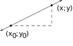
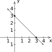
In Section A.3.2, we concerned ourselves with the finite line segment between two points and . Specifically, we found its length (the distance between and ) and its midpoint. In this section, our focus will be on the entire line, and ways to describe it algebraically. Consider the generic situation below.
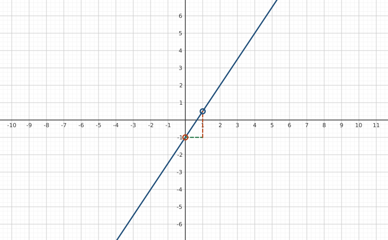
Interactive figurey = mx + b: b is where the line starts, m is rise over a run of oneDrag the Slope m and Intercept b sliders.
XYZ Graph · viewer build 5edf91b
The line is y = mx + b with both letters on sliders. The marked point (0, b) is the y-intercept, where the line meets the vertical axis; from it the dashed green run of exactly one unit and the dashed rust rise of exactly m units reach the second marked point (1, m + b), so the rise of this unit triangle is the slope itself. Slide b and the line moves up or down without tilting; slide m and it pivots about the intercept, the rise leg growing, shrinking, and flipping below the run when m is negative.Figure 15.62
To give a sense of the `steepness' of the line, we recall that we can compute the slope of the line as follows. (Read the character as `change in'.)
A couple of notes about Equation A.3 are in order. First, don't ask why we use the letter `' to represent slope. There are many explanations out there, but apparently no one really knows for sure.1 Secondly, the stipulation (or ) ensures that we aren't trying to divide by zero. The reader is invited to pause to think about what is happening geometrically when the `change in ' is ; the anxious reader can skip along to the next example.
A few comments about Example A.5.1 are in order. First, if the slope is positive then the resulting line is said to be `increasing', meaning as we move from left to right,2 the -values are getting larger.3 Similarly, if the slope is negative, we say the line is `decreasing', since as we move from left to right, the -values are getting smaller. A slope of results in a horizontal line which we say is `constant', since the -values here remain unchanged as we move from left to right, and an undefined slope results in a vertical line.4
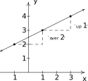
Second, the larger the slope is in absolute value, the steeper the line. You may recall from Intermediate Algebra that slope can be described as the ratio `'. For example, if the slope works out to be , we can interpret this as a `rise' of unit upward for every `run' of units to the right:
Figure 15.69
In this way, we may view the slope as `the rate of change of with respect to '. From the expression
we get so that the -values change `' times as fast as the -values. We'll have more to say about this concept in Section 1.2 when we explore applications of linear functions; presently, we will keep our attention focused on the analytic geometry of lines. To that end, our next task is to find algebraic equations that describe lines and we start with a discussion of vertical and horizontal lines.
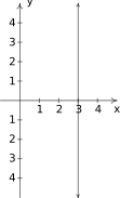
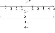
Consider the two lines shown below: (for `V'ertical Line) and (for `H'orizontal Line).
Figure 15.70The line Figure 15.71The line
All of the points on the line have an -coordinate of . Conversely, any point with an -coordinate of lies on the line . Said differently, the point lies on if and only if . Because of this, we say the equation
describes the line , or, said differently, the graph of the equation is the line .
In Section 5.5, we'll spend a great deal of time talking about graphing equations. For now, it suffices to know that a graph of an equation is a plot of all of the points which make the equation true. So to graph , we plot all of the points which satisfy and this gives us our vertical line .
Turning our attention to , we note that every point on has a -coordinate of , and vice-versa. Hence the equation describes the line , or the graph of the equation is . In general:
Of course, we may be working on axes which aren't labeled with the `usual' 's and 's. In this case, we understand Equation A.4 to say `' describes a vertical line through and `' describes a horizontal line through .
Using the concept of slope, we can develop equations for the other varieties of lines. Suppose a line has a slope of and contains the point . Suppose is another point on the line, as indicated below.
Figure 15.76
Equation A.3 yields
which is known as the point-slope form of a line.
A few remarks about Equation A.5 are in order. First, note that if the slope , then the line is horizontal and Equation A.5 reduces to or , as prescribed by Equation A.4.5 Second, we may need to change the letters in Equation A.5 from `' and `' depending on the context, so while Equation A.5 should be committed to memory, it should be understood that `' refers to whichever variable is used to label the horizontal axis, and refers to whichever variable is used to label the vertical axis. Lastly, while Equation A.5 is, by far, the easiest way to construct the equation of a line given a point and a slope, more often than not, the equation is solved for and simplified into the form below.
Equation A.6 is probably6 a familiar sight from Intermediate Algebra. You may recall from that class that the `intercept' in `slope-intercept' comes from the fact that this line `intercepts' or crosses the -axis at the point .7 If we set the slope, , we obtain , the formula for Horizontal Lines first introduced in Equation A.4. Hence, any line which has a defined slope can be represented in both point-slope and slope-intercept forms. The only exceptions are vertical lines.8 There is one equation - the aptly named 'general form' - which describes every type of line and it is presented on the next page.
Note the indefinite article `a' in Equation A.7. The line is a general form for the horizontal line through , but so are and . The reader is left to ponder the use of the definite article `the' in Equations A.5 and A.6. Regardless of which form the equation of a line takes, note that the variables involved are all raised to the first power.9 For instance, there are no terms, no terms or any variables appearing in denominators. Let's look at a few examples.
While every point on a line holds value and meaning,11 we've reminded you of certain points, called `intercepts,' which hold special enough significance to be singled out. Formally, we define these as follows.
As usual, the labels of the axes in the problem will dictate the labels on the intercepts. If we're working in the -plane, for instance, there would be - and -intercepts.
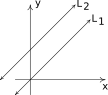
The last little bit of analytic geometry we need to review about lines are the concepts of `parallel' and `perpendicular' lines. Parallel lines do not intersect,12 and hence, parallel lines necessarily have the same slope. Perpendicular lines intersect at a right () angle. The relationship between these slopes is somewhat more complicated, and is summarized below.
Figure 15.80, Figure 15.81,
A few remarks about Theorem A.3 are in order. First off, the theorem assumes that the slopes of the lines exist. The reader is encouraged to think about the case when one (or both) of the slopes don't exist. Along those same lines, the reader is encouraged to think about why the stipulations and appear in the statement regarding slopes of perpendicular lines, and what happens in this case as well. (Think geometrically!) In Exercise, you'll prove the assertion about the slopes of perpendicular lines. For now, we accept it as true and use it in the following example.
Our last example with lines sets up a fourth kind of symmetry which will be revisited in Section 5.6.
Exercises
In Exercises -, find both the point-slope form and the slope-intercept form of the line with the given slope which passes through the given point.
In Exercises -, find the slope-intercept form of the line which passes through the given points.
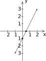
In Exercises -, graph the line. Find the slope, -intercept and -intercept, if any exist.
Graph on both the - and -axes. What characteristics to both graphs share? What's different?
Find all of the points on the line which are units from the point .
In Exercises -, you are given a line and a point which is not on that line. Find the line parallel to the given line which passes through the given point.
In Exercises -, you are given a line and a point which is not on that line. Find the line perpendicular to the given line which passes through the given point.
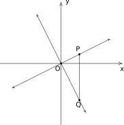
We shall now prove that is perpendicular to if and only if . To make our lives easier we shall assume that and . We can also “move” the lines so that their point of intersection is the origin without messing things up, so we'll assume (Take a moment with your classmates to discuss why this is okay.) Graphing the lines and plotting the points , and gives us the following set up.
Figure 15.85
The line will be perpendicular to the line if and only if is a right triangle. Let be the distance from to , let be the distance from to and let be the distance from to . Use the Pythagorean Theorem to show that is a right triangle if and only if by showing if and only if .
Answers
slope:
-intercept:
-intercept:
Figure 15.86
slope:
-intercept:
-intercept:
Figure 15.87
slope:
-intercept:
-intercept: none
Figure 15.88
slope:
-intercept:
-intercept:
Figure 15.89
slope:
-intercept:
-intercept:
Figure 15.90
slope:
-intercept:
-intercept:
Figure 15.91
slope:
-intercept:
-intercept:
Figure 15.92
slope:
-intercept:
-intercept:
Figure 15.93
and
Adapted from Precalculus with Integrated Calculus, edition 4i, by Carl Stitz and Jeff Zeager (stitz-zeager.com), licensed under CC BY-NC-SA 3.0. Changes were made: reformatted as an accessible XYZ web edition. License: CC-BY-NC-SA-3.0.
These eBooks are a prerelease and are not yet certified conformant with WCAG 2.1 AA or any other accessibility standard. Every page is built against an automated accessibility gate, and our target for the published editions is WCAG 2.2 Level AA. If something is unusable, please tell us.