
7.6 Applications of Exponential and Logarithmic Functions
As we mentioned in Sections 7.1 and 7.2, exponential and logarithmic functions are used to model a wide variety of behaviors in the real world. In the examples that follow, note that while the applications are drawn from many different disciplines, the mathematics remains essentially the same. Due to the applied nature of the problems we will examine in this section, we will often express our final answers as decimal approximations (after finding exact answers first, of course!)
Applications of Exponential Functions
Perhaps the most well-known application of exponential functions comes from the financial world. Suppose you have to invest at your local bank and they are offering a whopping annual percentage interest rate. This means that after one year, the bank will pay you of that , or in interest, so you now have . This is in accordance with the formula for simple interest which you have undoubtedly run across at some point before.
Suppose, however, that six months into the year, you hear of a better deal at a rival bank.2 Naturally, you withdraw your money and try to invest it at the higher rate there. Since six months is one half of a year, that initial yields in interest.
You take your off to the competitor and find out that those restrictions which may apply actually do apply, so you return to your bank and re-deposit the for the remaining six months of the year.
To your surprise and delight, at the end of the year your statement reads , not as you had expected.3 Where did those extra six cents come from?
For the first six months of the year, interest was earned on the original principal of , but for the second six months, interest was earned on , that is, you earned interest on your interest. This is the basic concept behind compound interest.
In the previous discussion, we would say that the interest was compounded twice per year, or semiannually.4 If more money can be earned by earning interest on interest already earned, one wonders what happens if the interest is compounded more often, say every three months - times a year, or `quarterly.'
In this case, the money is in the account for three months, or of a year, at a time. After the first quarter, we have . We now invest the for the next three months and find that at the end of the second quarter, we have . Continuing in this manner, the balance at the end of the third quarter is , and, at last, we obtain . The extra two cents hardly seems worth it, but we see that we do in fact get more money the more often we compound.
In order to develop a formula for this phenomenon, we need to do some abstract calculations. Suppose we wish to invest our principal at an annual rate and compound the interest times per year. This means the money sits in the account of a year between compoundings. Let denote the amount in the account after the compounding.
Then which simplifies to . After the second compounding, we use as our new principal and get . Continuing in this fashion, we get , , and so on, so that .
Since we compound the interest times per year, after years, we have compoundings. We have just derived the general formula for compound interest below.
If we take , , and , Equation 7.2 becomes which reduces to . To check this new formula against our previous calculations, we find , , , and .
We have observed that the more times you compound the interest per year, the more money you will earn in a year. Let's push this notion to the limit.8
Consider an investment of invested at interest for year compounded times a year. Equation 7.2 tells us that the amount of money in the account after year is . Below is a table of values relating and .
As promised, the more compoundings per year, the more money there is in the account, but we also observe that the increase in money is greatly diminishing.
We are witnessing a mathematical `tug of war'. While we are compounding more times per year, and hence getting interest on our interest more often, the amount of time between compoundings is getting smaller and smaller, so there is less time to build up additional interest.
With Calculus, we can show9 that , where is the natural base first presented in Section 7.1. Taking the number of compoundings per year to infinity results in what is called continuously compounded interest.
Using the limit definition of along with some limit properties, we can derive a general formula for continuously compounded interest.
Consider the limit . In order to use the limit definition of `,' we need to make a substitution to make `' look like `.'
If we let , we get , so and . In the context of compound interest, , so implies and vice-versa so the limit becomes:
Using Properties of Limits, Theorem 6.2, we get:
A couple of remarks are in order. First, in the limit , the variable here, , takes on natural number values, and as such, is a discrete variable, not a continuous one.10 We'll revisit limits of discrete variables in Section 10.1.1.
Second, when we use the limit definition of `' in the above argument, we used . Like , the variable is a discrete variable (not necessarily natural numbers, but discrete nonetheless). Since both and are tending to infinity, this change in dummy variable doesn't affect the limit.11
Last, we note that the Real Numbers Power rule applies since . We codify this result in the following theorem.
It is worth noting that if we take the scenario of Example 7.6.1 and compare monthly compounding to continuous compounding over years, we find that monthly compounding yields which is about , whereas continuously compounding gives which is about - a difference of less than .
Equations 7.2 and both use exponential functions to describe the growth of an investment. It turns out, the same principles which govern compound interest are also used to model short term growth of populations. As with many concepts in this text, these notions are best formalized using the language of Calculus. Nevertheless, we do our best here.
In Biology, The Law of Uninhibited Growth states as its premise that the instantaneous rate at which a population increases at any time is directly proportional to the population at that time. In other words, the more organisms there are at a given moment, the faster they reproduce. Formulating the law as stated results in a differential equation, which requires Calculus to solve. Solving said differential equation gives us the formula below.
It is worth taking some time to compare Equations and 7.4. In Equation, we use to denote the initial investment; in Equation 7.4, we use to denote the initial population. In Equation, denotes the annual interest rate, and so it shouldn't be too surprising that the in Equation 7.4 corresponds to a growth rate as well. While Equations and 7.4 look entirely different, they both represent the same mathematical concept.
Whereas Equations and 7.4 model the growth of quantities, we can use equations like them to describe the decline of quantities.
One example we've seen already is Example 7.1.2 in Section 7.1. There, the value of a car decreased from its purchase price of to nothing at all.
Another real world phenomenon which follows suit is radioactive decay. There are elements which are unstable and emit energy spontaneously. In doing so, the amount of the element itself diminishes.
The assumption behind this model is that the rate of decay of an element at a particular time is directly proportional to the amount of the element present at that time. In other words, the more of the element there is, the faster the element decays.
This is precisely the same kind of hypothesis which drives The Law of Uninhibited Growth, and as such, the equation governing radioactive decay is hauntingly similar to Equation 7.4 with the exception that the rate constant is negative.
We now turn our attention to some more mathematically sophisticated models. One such model is Newton's Law of Cooling, which we first encountered in Example 7.1.3 of Section 7.1.
In that example we had a cup of coffee cooling from to room temperature according to the formula , where was measured in minutes. In that situation, we knew the physical limit of the temperature of the coffee was room temperature,14 and the differential equation which gives rise to our formula for takes this into account.
Whereas the radioactive decay model had a rate of decay at time directly proportional to the amount of the element which remained at time , Newton's Law of Cooling states that the rate of cooling of the coffee at a given time is directly proportional to how much of a temperature gap exists between the coffee at time and room temperature, not the temperature of the coffee itself. In other words, the coffee cools faster when it is first served, and as its temperature nears room temperature, the coffee cools ever more slowly.
Of course, if we take an item from the refrigerator and let it sit out in the kitchen, the object's temperature will rise to room temperature, and since the physics behind warming and cooling is the same, we combine both cases in the equation below.
If we re-examine the situation in Example 7.1.3 with , , and , we get, according to Equation 7.6, which reduces to the original formula given in that example. The rate constant in this case indicates the coffee is cooling at a rate equal to of the difference between the temperature of the coffee and its surroundings.
Note in Equation 7.6 that the constant is positive for both the cooling and warming scenarios. What determines if the function is increasing or decreasing is if (the initial temperature of the object) is greater than (the ambient temperature) or vice-versa, as we see in our next example.
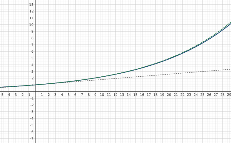
If we had taken the time to graph in Example 7.6.4, we would have found the horizontal asymptote to be , which corresponds to the temperature of the oven. We can also arrive at this conclusion analytically by applying `number sense'.
As , so that . The larger the value of , the smaller becomes so that , which suggests the graph of is approaching its horizontal asymptote from below. Physically, this means the roast will eventually warm up to .16
The function in this situation is sometimes called a limited growth model, since the function remains bounded as . If we apply the principles behind Newton's Law of Cooling to a biological example, it says the growth rate of a population is directly proportional to how much room the population has to grow. In other words, the more room for expansion, the faster the growth rate.
Our final model, the logistic growth model combines The Law of Uninhibited Growth with limited growth and states that the rate of growth of a population varies jointly with the population itself as well as the room the population has to grow.
The logistic function is used not only to model the growth of organisms, but is also often used to model the spread of disease and rumors.18
If we take the time to analyze the graph of in Example 7.6.5, we can see graphically how logistic growth combines features of uninhibited and limited growth.
We can see graphically that there is an inflection point in the graph. In this case, the inflection point is called the point of diminishing returns. Even though the function is still increasing through the inflection point (more people are hearing the rumor), the rate at which it does so begins to decrease.
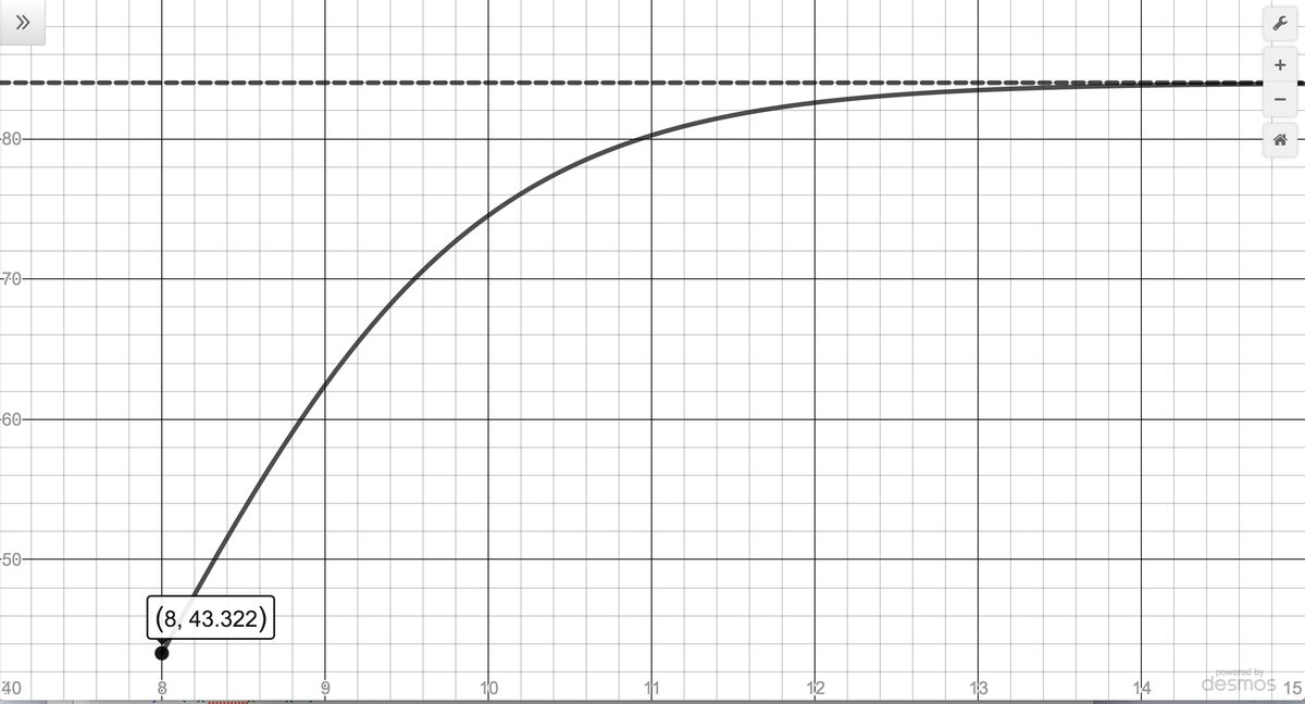
With Calculus, one can show the point of diminishing returns always occurs at half the limiting population.21 (In our case, when .) So with that in mind, we present two portions of the graph of , one on the interval , the other on . The former looks strikingly like uninhibited growth while the latter like limited growth.
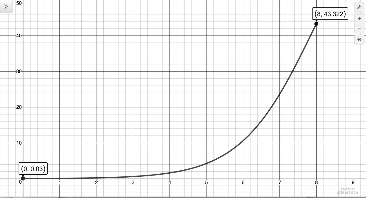
for
for
Applications of Logarithms
Just as many physical phenomena can be modeled by exponential functions, the same is true of logarithmic functions. In Exercises, and of Section 7.2, we showed that logarithms are useful in measuring the intensities of earthquakes (the Richter scale), sound (decibels) and acids and bases (pH). We now present yet a different use of the a basic logarithm function, password strength .
Chemical systems known as buffer solutions have the ability to adjust to small changes in acidity to maintain a range of pH values. Buffer solutions have a wide variety of applications from maintaining a healthy fish tank to regulating the pH levels in blood. Our next example shows how the pH in a buffer solution is a little more complicated than the pH we first encountered in Exercise in Section 7.2.
Another place logarithms are used is in data analysis. Suppose, for instance, we wish to model the spread of influenza A (H1N1), the so-called `Swine Flu'. Below is data taken from the World Health Organization ( WHO ) where represents the number of days since April 28, 2009, and represents the number of confirmed cases of H1N1 virus worldwide.
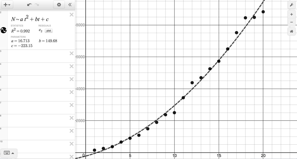
Making a scatter plot of the data treating as the independent variable and as the dependent variable gives the plot below on the left. Which models are suggested by the shape of the data?
Thinking back Section 1.4, we try a Quadratic Regression. We find with , indicating a pretty good fit. However, is there any underlying scientific principle which would account for these data to be quadratic? Are there other models which fit the data better?
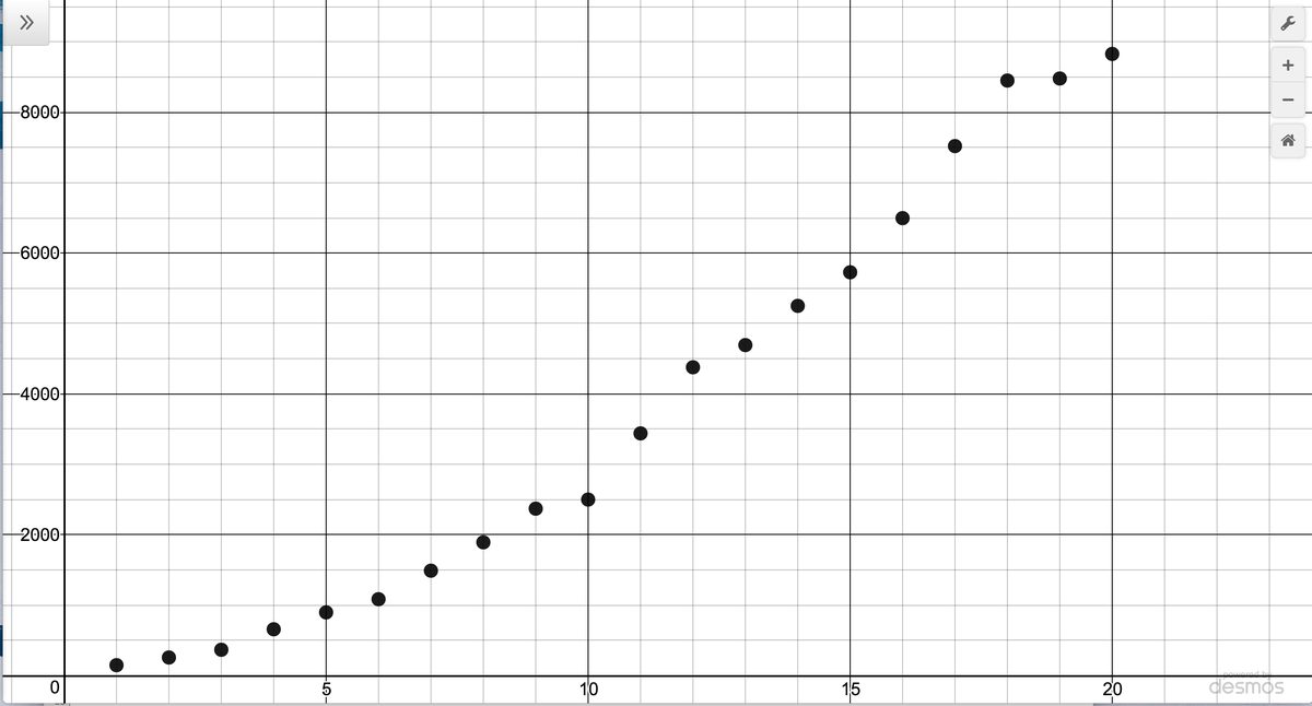
Scatterplot of the Data
A quadratic regression model
To answer these questions, scientists often use logarithms in an attempt to `linearize' non-liner data sets such as the one before us. To see how this could work, suppose we guessed the relationship between and is something from Section 4.2, .
By taking the natural logs of both sides and using the Product and Power Rules, in turn, we find that . If we let and , the model takes the form which is a linear model with slope and -intercept . So, instead of plotting versus , we plot versus and find a linear regression for this data set.
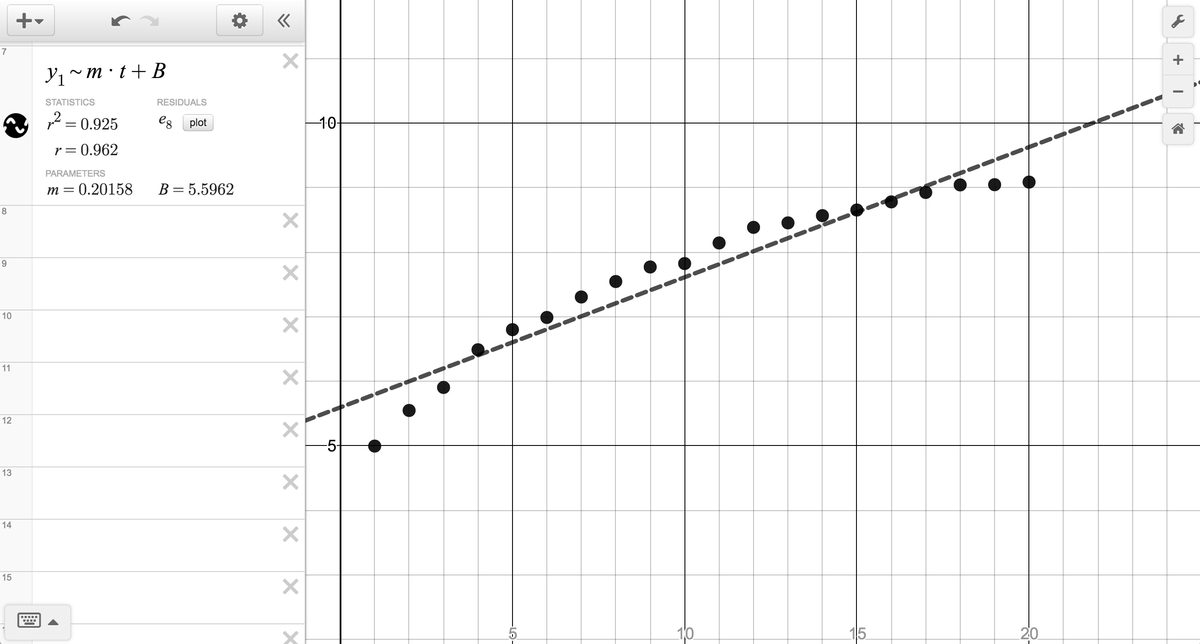
linear regression:
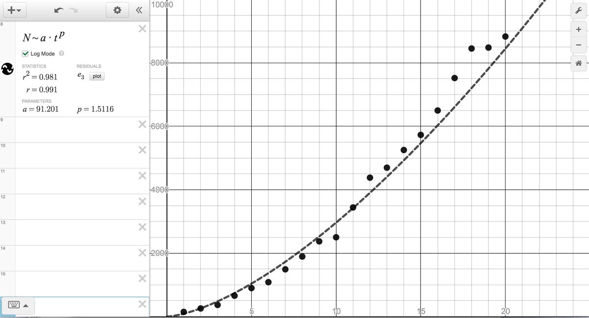
power function regression:
We see , which is very close to indicating a very good fit. The slope of the regression line is which corresponds to our exponent . The -intercept corresponds to , so that . Hence, we get the model .
Of interest here is that the graphing utility we used, desmos has its own built-in power regression model. If the `log mode' square is checked, the graphing utility returns the same model we obtained using our linearization (since the routine which determines the coefficients uses logarithms as well.)25
At this point, the quadratic model fits the data better, ostensibly because we have three parameters we can adjust in the formula to minimize our error as opposed to just two parameters in the formula . Neither model, however, is based on any underlying scientific principle.
If we think about this situation from a scientific perspective, it does seem to make sense that, at least in the early stages of the outbreak, the more people who have the flu, the faster it will spread. This suggests we fit the data to an uninhibited growth model.
As written, Equation 7.4 gives uninhibited growth as . Here, for simplicity's sake, we relabel and so that we are looking for parameters and so that .
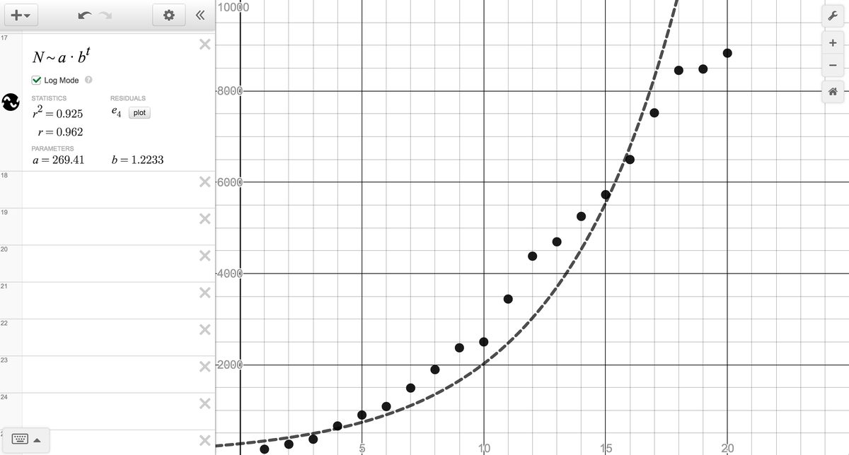
If we assume then, taking logs as before, we get . If we let , then, once again, we get a linear model this time with slope and -intercept . We present the results of the regression below. While there is a strong correlation, , the plot doesn't instill the greatest of confidence in this model.
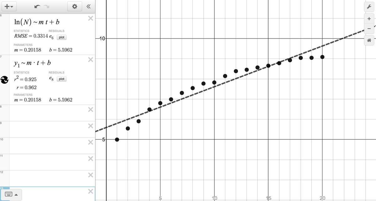
linear regression:
exponential regression:
From the slope of the model, we have so . From the -intercept of the model, we get so , so that our model is . Using the built-in exponential regression (again, with `log mode' checked) returns the model , the discrepancy between and stemming ostensibly from round-off error.
The exponential model didn't fit the data as well as the quadratic or power function model, but it stands to reason that, perhaps, the spread of the flu is not unlike that of the spread of a rumor and that a logistic model can be used to model the data. Again, for simplicity, we abbreviate the model given in Equation 7.7 from to .
Running the data, a logistic function appears to be an excellent fit, both judging by the graph as well as the coefficient of determination, . Moreover, the underlying principles which lead to the formulation of this model seem reasonable enough.
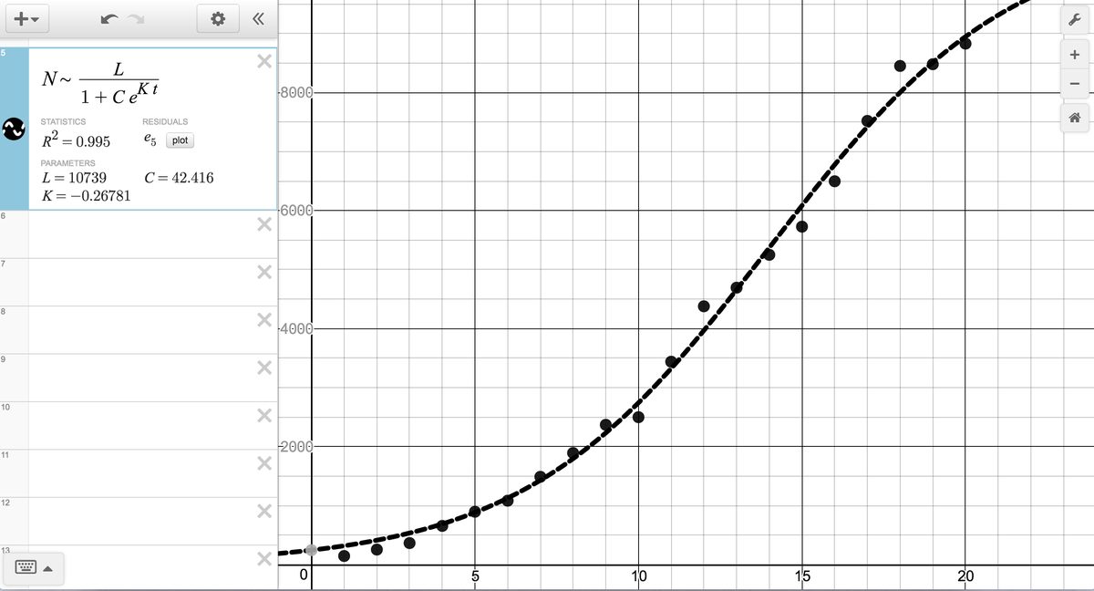
While the quadratic model also fits extremely well, our logistic model takes into account that only a finite number of people will ever get the flu (according to our model, ), whereas the quadratic model predicts no limit to the number of cases. As we have stated several times before in the text, mathematical models, regardless of their sophistication, are just that: models, and they all have their limitations.26
Exercises
For each of the scenarios given in Exercises -,
- Find the amount in the account as a function of the term of the investment in years.
- To the nearest cent, determine how much is in the account after , , and years.
- To the nearest year, determine how long will it take for the initial investment to double.
- Find and interpret the average rate of change of the amount in the account from the end of the fourth year to the end of the fifth year, and from the end of the thirty-fourth year to the end of the thirty-fifth year. Round your answer to two decimal places.
- is invested in an account which offers , compounded monthly.
- is invested in an account which offers , compounded continuously.
- is invested in an account which offers , compounded monthly.
- is invested in an account which offers , compounded continuously.
- is invested in an account which offers , compounded monthly.
- is invested in an account which offers , compounded continuously.
- Look back at your answers to Exercises -. What can be said about the difference between monthly compounding and continuously compounding the interest in those situations? With the help of your classmates, discuss scenarios where the difference between monthly and continuously compounded interest would be more dramatic. Try varying the interest rate, the term of the investment and the principal. Use computations to support your answer.
- How much money needs to be invested now to obtain in 3 years if the interest rate in a savings account is , compounded continuously? Round your answer to the nearest cent.
- How much money needs to be invested now to obtain in 10 years if the interest rate in a CD is , compounded monthly? Round your answer to the nearest cent.
On May, 31, 2009, the Annual Percentage Rate listed at Jeff's bank for regular savings accounts was compounded monthly. Use Equation 7.2 to answer the following.
- If what is ?
- Solve the equation for .
- What principal should be invested so that the account balance is $2000 is three years?
Jeff's bank also offers a 36-month Certificate of Deposit (CD) with an APR of .
- If what is ?
- Solve the equation for .
- What principal should be invested so that the account balance is $2000 in three years?
- The Annual Percentage Yield is the simple interest rate that returns the same amount of interest after one year as the compound interest does. With the help of your classmates, compute the APY for this investment.
- A finance company offers a promotion on loans. The borrower does not have to make any payments for the first three years, however interest will continue to be charged to the loan at compounded continuously. What amount will be due at the end of the three year period, assuming no payments are made? If the promotion is extended an additional three years, and no payments are made, what amount would be due?
- Use Equation 7.2 to show that the time it takes for an investment to double in value does not depend on the principal , but rather, depends only on the APR and the number of compoundings per year. Let and with the help of your classmates compute the doubling time for a variety of rates . Then look up the Rule of 72 and compare your answers to what that rule says. If you're really interested27 in Financial Mathematics, you could also compare and contrast the Rule of 72 with the Rule of 70 and the Rule of 69.
In Exercises -, we list some radioactive isotopes and their associated half-lives. Assume that each decays according to the formula where is the initial amount of the material and is the decay constant. For each isotope:
- Find the decay constant . Round your answer to four decimal places.
- Find a function which gives the amount of isotope which remains after time . (Keep the units of and the same as the given data.)
- Determine how long it takes for of the material to decay. Round your answer to two decimal places. (HINT: If of the material decays, how much is left?)
- Cobalt 60, used in food irradiation, initial amount 50 grams, half-life of years.
- Phosphorus 32, used in agriculture, initial amount 2 milligrams, half-life days.
- Chromium 51, used to track red blood cells, initial amount 75 milligrams, half-life days.
- Americium 241, used in smoke detectors, initial amount 0.29 micrograms, half-life years.
- Uranium 235, used for nuclear power, initial amount kg, half-life million years.
- With the help of your classmates, show that the time it takes for of each isotope listed in Exercises - to decay does not depend on the initial amount of the substance, but rather, on only the decay constant . Find a formula, in terms of only, to determine how long it takes for of a radioactive isotope to decay.
- In Example 7.1.2 in Section 7.1, the exponential function was used to model the value of a car over time. Use a change of base formula to rewrite the model in the form .
The Gross Domestic Product (GDP) of the US (in billions of dollars) years after the year 2000 can be modeled by:
- Find and interpret .
- According to the model, what should have been the GDP in 2007? In 2010? (According to the US Department of Commerce , the 2007 GDP was billion and the 2010 GDP was billion.)
The diameter of a tumor, in millimeters, days after it is detected is given by:
- What was the diameter of the tumor when it was originally detected?
- How long until the diameter of the tumor doubles?
Under optimal conditions, the growth of a certain strain of E. Coli is modeled by the Law of Uninhibited Growth where is the initial number of bacteria and is the elapsed time, measured in minutes. From numerous experiments, it has been determined that the doubling time of this organism is 20 minutes. Suppose 1000 bacteria are present initially.
- Find the growth constant . Round your answer to four decimal places.
- Find a function which gives the number of bacteria after minutes.
- How long until there are 9000 bacteria? Round your answer to the nearest minute.
Yeast is often used in biological experiments. A research technician estimates that a sample of yeast suspension contains 2.5 million organisms per cubic centimeter (cc). Two hours later, she estimates the population density to be 6 million organisms per cc. Let be the time elapsed since the first observation, measured in hours. Assume that the yeast growth follows the Law of Uninhibited Growth .
- Find the growth constant . Round your answer to four decimal places.
- Find a function which gives the number of yeast (in millions) per cc after hours.
- What is the doubling time for this strain of yeast?
- The Law of Uninhibited Growth also applies to situations where an animal is re-introduced into a suitable environment. Such a case is the reintroduction of wolves to Yellowstone National Park. According to the National Park Service , the wolf population in Yellowstone National Park was 52 in 1996 and 118 in 1999. Using these data, find a function of the form which models the number of wolves years after 1996. (Use to represent the year 1996. Also, round your value of to four decimal places.) According to the model, how many wolves were in Yellowstone in 2002? (The recorded number is 272.)
- During the early years of a community, it is not uncommon for the population to grow according to the Law of Uninhibited Growth. According to the Painesville Wikipedia entry, in 1860, the Village of Painesville had a population of 2649. In 1920, the population was 7272. Use these two data points to fit a model of the form were is the number of Painesville Residents years after 1860. (Use to represent the year 1860. Also, round the value of to four decimal places.) According to this model, what was the population of Painesville in 2010? (The 2010 census gave the population as 19,563) What could be some causes for such a vast discrepancy? For more on this, see Exercise.
The population of Sasquatch in Bigfoot county is modeled by
where is the population of Sasquatch years after .
- Find and interpret .
- Find the population of Sasquatch in Bigfoot county in 2013 rounded to the nearest Sasquatch.
- To the nearest year, when will the population of Sasquatch in Bigfoot county reach 60?
- Find and interpret analytically. Check your answer using a graphing utility.
Let .
- From Calculus, we know the inflection point of the graph of is . This means the function is increasing the fastest at , or, equivalently, the slope at is the largest anywhere on the graph. Graph using a graphing utility and convince yourself of the reasonableness of this claim.
Find average rate of change of over each of the intervals below. What do you guess the slope of the curve is at ? Zoom in on the graph near to check your guess.
The half-life of the radioactive isotope Carbon-14 is about 5730 years.
- Use Equation 7.5 to express the amount of Carbon-14 left from an initial milligrams as a function of time in years.
- What percentage of the original amount of Carbon-14 is left after 20,000 years?
- If an old wooden tool is found in a cave and the amount of Carbon-14 present in it is estimated to be only 42% of the original amount, approximately how old is the tool?
- Radiocarbon dating is not as easy as these exercises might lead you to believe. With the help of your classmates, research radiocarbon dating and discuss why our model is somewhat over-simplified.
- Carbon-14 cannot be used to date inorganic material such as rocks, but there are many other methods of radiometric dating which estimate the age of rocks. One of them, Rubidium-Strontium dating, uses Rubidium-87 which decays to Strontium-87 with a half-life of 50 billion years. Use Equation 7.5 to express the amount of Rubidium-87 left from an initial 2.3 micrograms as a function of time in billions of years. Research this and other radiometric techniques and discuss the margins of error for various methods with your classmates.
- Find and interpret the relative rate of change of in Equation 7.2 over the interval .
- Use Equation 7.5 to show that where is the half-life of the radioactive isotope.
A pork roast28 was taken out of a hardwood smoker when its internal temperature had reached F and it was allowed to rest in a F house for 20 minutes after which its internal temperature had dropped to F.
Assuming that the temperature of the roast follows Newton's Law of Cooling (Equation 7.6),
- Express the temperature (in F) as a function of time (in minutes).
- Find the time at which the roast would have dropped to F had it not been eaten.
In reference to Exercise in Section 4.2, if Fritzy the Fox's speed is the same as Chewbacca the Bunny's speed, Fritzy's pursuit curve is given by
Graph this path for using a graphing utility. Investigate and interpret.
- The current measured in amps in a certain electronic circuit with a constant impressed voltage of 120 volts is given by where is the number of seconds after the circuit is switched on. Determine . (This is called the steady state current.)
If the voltage in the circuit in Exercise above is switched off after 30 seconds, the current is given by the piecewise-defined function
With the help of a graphing utility, graph and discuss with your classmates the physical significance of the two parts of the graph and .
In Exercise in Section 1.4, we stated that the cable of a suspension bridge formed a parabola but that a free hanging cable did not. A free hanging cable forms a catenary and its basic shape is given by . Use a graphing utility to graph this function. What are its domain and range? What is its end behavior? Is it invertible? How do you think it is related to the function given in Exercise in Section 7.4 and the one given in the answer to Exercise in Section 7.5?
When flipped upside down, the catenary makes an arch. The Gateway Arch in St. Louis, Missouri has the shape
where and are measured in feet and . Find the highest point on the arch.
In Exercise in Section 1.4, we examined the data set given below which showed how two cats and their surviving offspring can produce over 80 million cats in just ten years. Plot versus as was done on page using a graphing utility.
Find a linear model for this new data and comment on its goodness of fit and find an exponential model for the original data and comment on its goodness of fit.
Table 7.1 Year 1 2 3 4 5 6 7 8 9 10 Number of Cats 12 66 382 2201 12680 73041 420715 2423316 13968290 80399780 In Example 4.2.3 in Section 4.2, we fit a power function of the form to a set of data, . In this exercise, we use logs to linearize this data using the same methods presented on page, but with a slight difference in interpretation.
- Starting with , take natural logs of both sides of the equation and use log properties to rewrite the resulting equation as: .
Use a graphing utility to find a least squares regression line using the data .
NOTE: In this situation, we are plotting versus instead of versus .
- Find the slope of the regression line and the intercept . Use these to construct a model of the form . Find and interpret .
- Graph both the model obtained in Example 4.2.3 and the model obtained in part along with the original data. What do you notice?
This exercise is a follow-up to Exercise which more thoroughly explores the population growth of Painesville, Ohio. According to Wikipedia , the population of Painesville, Ohio is given by
Table 7.2 Year 1860 1870 1880 1890 1900 1910 1920 1930 1940 1950 Population 2649 3728 3841 4755 5024 5501 7272 10944 12235 14432 Table 7.3 Year 1960 1970 1980 1990 2000 Population 16116 16536 16351 15699 17503 - Use a graphing utility to perform an exponential regression on the data from 1860 through 1920 only, letting represent the year 1860 as before. How does this model compare with the model you found in Exercise ? Use the graphing utility's exponential model to predict the population in 2010. (The 2010 census gave the population as 19,563)
The logistic model fit to all of the given data points for the population of Painesville years after 1860 (again, using as 1860) is
According to this model, what should the population of Painesville have been in 2010? (The 2010 census gave the population as 19,563.) What is the population limit of Painesville?
According to OhioBiz , the census data for Lake County, Ohio is as follows:
Table 7.4 Year 1860 1870 1880 1890 1900 1910 1920 1930 1940 1950 Population 15576 15935 16326 18235 21680 22927 28667 41674 50020 75979 Table 7.5 Year 1960 1970 1980 1990 2000 Population 148700 197200 212801 215499 227511 - Use a graphing utility to fit a logistic model to these data with representing the year 1860.
- Graph the data and your model using a graphing utility to judge the reasonableness of the fit.
- Use this model to estimate the population of Lake County in 2010. (The 2010 census gave the population to be 230,041.)
- According to your model, what is the population limit of Lake County, Ohio?
According to facebook , the number of active users of facebook has grown significantly since its initial launch from a Harvard dorm room in February 2004. The chart below has the approximate number of active users, in millions, months after February 2004. For example, the first entry means that there were million active users in December 2004 and the last entry means that there were million active users in July 2010.
Table 7.6 Month 10 22 34 38 44 54 59 60 62 65 67 70 72 77 Active Users in Millions 1 5.5 12 20 50 100 150 175 200 250 300 350 400 500 With the help of your classmates, find a model for this data.
Each Monday during the registration period before the Fall Semester at LCCC, the Enrollment Planning Council gets a report prepared by the data analysts in Institutional Effectiveness and Planning.29 While the ongoing enrollment data is analyzed in many different ways, we shall focus only on the overall headcount. Below is a chart of the enrollment data for Fall Semester 2008. It starts 21 weeks before “Opening Day” and ends on “Day 15” of the semester, but we have relabeled the top row to be through so that the math is easier. (Thus, is Opening Day.)
Table 7.7 Week 1 2 3 4 5 6 7 8 Total Headcount 1194 1564 2001 2475 2802 3141 3527 3790 Table 7.8 Week 9 10 11 12 13 14 15 16 Total Headcount 4065 4371 4611 4945 5300 5657 6056 6478 Table 7.9 Week 17 18 19 20 21 22 23 24 Total Headcount 7161 7772 8505 9256 10201 10743 11102 11181 With the help of your classmates, find a model for this data. Unlike most of the phenomena we have studied in this section, there is no single differential equation which governs the enrollment growth. Thus there is no scientific reason to rely on a logistic function even though the data plot may lead us to that model. What are some factors which influence enrollment at a community college and how can you take those into account mathematically?
When we wrote this exercise, the Enrollment Planning Report for Fall Semester 2009 had only 10 data points for the first 10 weeks of the registration period. Those numbers are given below.
Table 7.10 Week 1 2 3 4 5 6 7 8 9 10 Total Headcount 1380 2000 2639 3153 3499 3831 4283 4742 5123 5398 With the help of your classmates, find a model for this data and make a prediction for the Opening Day enrollment as well as the Day 15 enrollment. (WARNING: The registration period for 2009 was one week shorter than it was in 2008 so Opening Day would be and Day 15 is .)
Answers
- , , ,
- It will take approximately years for the investment to double.
- The average rate of change from the end of the fourth year to the end of the fifth year is approximately . This means that the investment is growing at an average rate of per year at this point. The average rate of change from the end of the thirty-fourth year to the end of the thirty-fifth year is approximately . This means that the investment is growing at an average rate of per year at this point.
- , , ,
- It will take approximately years for the investment to double.
- The average rate of change from the end of the fourth year to the end of the fifth year is approximately . This means that the investment is growing at an average rate of per year at this point. The average rate of change from the end of the thirty-fourth year to the end of the thirty-fifth year is approximately . This means that the investment is growing at an average rate of per year at this point.
- , , ,
- It will take approximately years for the investment to double.
- The average rate of change from the end of the fourth year to the end of the fifth year is approximately . This means that the investment is growing at an average rate of per year at this point. The average rate of change from the end of the thirty-fourth year to the end of the thirty-fifth year is approximately . This means that the investment is growing at an average rate of per year at this point.
- , , ,
- It will take approximately years for the investment to double.
- The average rate of change from the end of the fourth year to the end of the fifth year is approximately . This means that the investment is growing at an average rate of per year at this point. The average rate of change from the end of the thirty-fourth year to the end of the thirty-fifth year is approximately . This means that the investment is growing at an average rate of per year at this point.
- , , ,
- It will take approximately years for the investment to double.
- The average rate of change from the end of the fourth year to the end of the fifth year is approximately . This means that the investment is growing at an average rate of per year at this point. The average rate of change from the end of the thirty-fourth year to the end of the thirty-fifth year is approximately . This means that the investment is growing at an average rate of per year at this point.
- , , ,
- It will take approximately years for the investment to double.
- The average rate of change from the end of the fourth year to the end of the fifth year is approximately . This means that the investment is growing at an average rate of per year at this point. The average rate of change from the end of the thirty-fourth year to the end of the thirty-fifth year is approximately . This means that the investment is growing at an average rate of per year at this point.
- years
- years
- so the APY is 2.27%
- ,
- years.
- days.
- days.
- years.
- million years, or billion years.
- This means that the GDP of the US in 2000 was billion dollars.
- and , so the model predicted a GDP of billion in 2007 and billion in 2010.
- , so the tumor was 15 millimeters in diameter when it was first detected.
- days.
- minutes
- hours
- , , . .
- , , . , so the population of Painesville in 2010 based on this model would have been 32,923.
- . There are 29 Sasquatch in Bigfoot County in 2010.
- Sasquatch.
- years.
- We find . As time goes by, the Sasquatch Population in Bigfoot County will approach 120. Graphically, has a horizontal asymptote .
The average rates of change are listed in order below. They suggest slope at is .
- so about 8.9% remains
- years old
- The relative rate of change of over is which is the annual percentage rate divided by the number of compoundings per year – that is, the percentage growth rate over one compounding.
- The roast would have cooled to F in about 95 minutes.
From the graph, it appears that . This is due to the presence of the term in the function. This means that Fritzy will never catch Chewbacca, which makes sense since Chewbacca has a head start and Fritzy only runs as fast as he does.
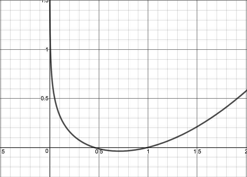
Figure 7.113 - The steady state current is 2 amps.
- 630 feet.
The linear regression on the data below is with .
This is an excellent fit.
Table 7.11 1 2 3 4 5 6 7 8 9 10 2.4849 4.1897 5.9454 7.6967 9.4478 11.1988 12.9497 14.7006 16.4523 18.2025 with . This is also an excellent fit and corresponds to our linearized model because .
- The linearized model is: with an .
- . meaning the bottom of wage earners take home of the total national income. Said differently, according to this model, the top of wage earners take home of the total national income.
We graph our answer to Example 4.2.3 in Section 4.2, , below on the left. Below on the right is the model we derived in this exercise.
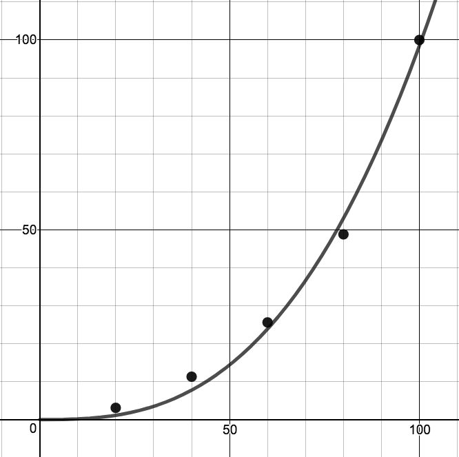
Figure 7.114 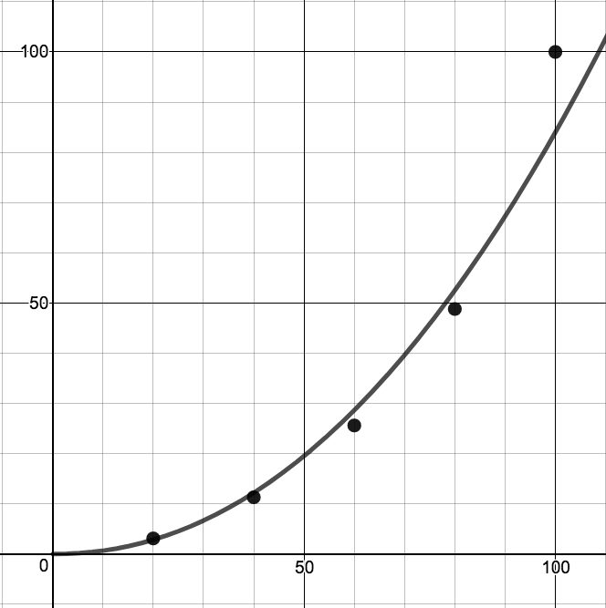
Figure 7.115
- We get: . Graphing this along with our answer from Exercise over the interval shows that they are pretty close. From this model, which once again overshoots the actual data value.
- , so this model predicts 17,914 people in Painesville in 2010, a more conservative number than was recorded in the 2010 census. We have , so the limiting population of Painesville based on this model is 18,691 people.
- , where is the number of years since 1860.
The plot of the data and the curve is below.
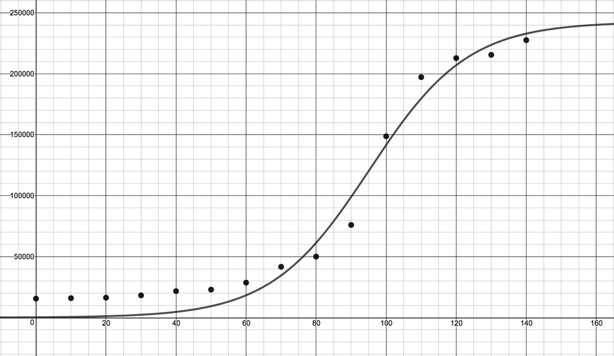
Figure 7.116 - , so this model predicts 232,884 people in Lake County in 2010.
- We get , so the limiting population of Lake County based on this model is 242,526 people.
Adapted from Precalculus with Integrated Calculus, edition 4i, by Carl Stitz and Jeff Zeager (stitz-zeager.com), licensed under CC BY-NC-SA 3.0. Changes were made: reformatted as an accessible XYZ web edition. License: CC-BY-NC-SA-3.0.