7.4 Equations and Inequalities involving Exponential Functions
In this section we will develop techniques for solving equations involving exponential functions. Consider the equation . After a moment's calculation, we find , so we have . The one-to-one property of exponential functions, detailed in Theorem 7.5, tells us that if and only if . This means that not only is a solution to , it is the only solution.
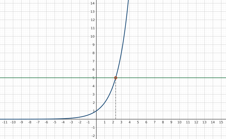
Interactive figureSolving a^x = c by sight: the crossing sits at x = log_a(c)Drag the Base a and Line height c sliders.
XYZ Graph · viewer build 5edf91b
The equation a^x = c asks where the exponential curve y = a^x crosses the horizontal line y = c. The marked crossing is the solution, and its x-coordinate is exactly log_a(c) = ln(c)/ln(a), which the dashed drop to the x-axis reads off. Slide the base a and the line height c: a larger base reaches the line sooner, a higher line pushes the crossing to the right, and a line at or below zero never meets the curve at all, which is the graphical face of the domain of the logarithm.
Now suppose we change the problem ever so slightly to . We could use one of the inverse properties of exponentials and logarithms listed in Theorem 7.4 to write . We'd then have , which means our solution is .
After all, the definition of is `the exponent we put on to get .' Indeed we could have obtained this solution directly by rewriting the equation in its logarithmic form . Either way, in order to get a reasonable decimal approximation to this number, we'd use the change of base formula, Theorem 7.8, to give us something more calculator friendly. Typically this means we convert our answer to base 10 or base , and we choose the latter: .
Still another way to obtain this answer is to `take the natural log' of both sides of the equation. Since is a function, as long as two quantities are equal, their natural logs are equal.1
We then use the Power Rule to write the exponent as a factor then divide both sides by the constant to obtain our answer.2
We summarize our two strategies for solving equations featuring exponential functions below.
Steps for Solving an Equation involving Exponential Functions
Isolate the exponential function.
If convenient, express both sides with a common base and equate the exponents.
Otherwise, take the natural log of both sides of the equation and use the Power Rule.
Note that verifying our solutions to the equations in Example 7.4.1analytically holds great educational value, since it reviews many of the properties of logarithms and exponents in tandem.
For example, to verify our solution to , we substitute and check:
We strongly encourage the reader to check the remaining equations analytically as well.
Since exponential functions are continuous on their domains, the Intermediate Value Theorem 2.14 applies. This allows us to solve inequalities using sign diagrams as demonstrated below.
We note here that while sign diagrams will always work for solving inequalities involving exponential functions, as we've seen previously, there are circumstances in which we can short-cut this method.
For example, consider number from Example 7.4.2 above: . Since the base , is an increasing function meaning it preserves inequalities.
We can use this to our advantage in this case and eliminate the exponential from the inequality altogether:
Hence, we've reduced our given inequality to . As seen in Section 1.4, we can solve this inequality by completing the square, graphing, or a sign diagram, whichever strikes the reader's fancy.
Our next example is a follow-up to Example 7.1.3 in Section 7.1.
We note that, once again, we can short-cut the sign diagram in Example 7.4.3 to solve . Since is increasing, it preserves inequality. This means we can solve this inequality as follows.
Since we are given , we arrive at the same answer or .
Note the importance, once again, of having a base larger than so that the corresponding logarithmic function is increasing. We can still adapt this strategy to exponential functions whose base is less than , but we need to remember the corresponding logarithmic function is decreasing so it reverses inequalities.
Our last example uses the tools of this section along with those developed in Section 6.3.
Note that the graph of produced by the graphing utility in Example 7.4.5 suggests the graph of has a horizontal asymptote as .
Indeed, it is the case that , however if we try to reason this analytically, we get another instance of an indeterminate form.9 As , but . Hence, as , we get the indeterminate form `.' Depending on how quickly the first factor approaches `' and how quickly the second factor approaches `', we could end up with `', `,' or some number in between.10
We'll explore more of this phenomenon in Exercise.11 For now, we take it as true that exponential functions dominate polynomial functions so in the above indeterminate form, the factor determines12 the end behavior of , so .
Exercises
In Exercises -, solve the equation analytically.
In Exercises -, solve the inequality analytically.
In Exercises -, use a graphing utility to help you solve the equation or inequality.
In Exercises -, find the domain of the function.
Since is a strictly increasing function, if then . Use this fact to solve the inequality without a sign diagram. Use this technique to solve the inequalities in Exercises -. (NOTE: Isolate the exponential function first!)
Compute the inverse of . State the domain and range of both and .
In Example 7.4.4, we found that the inverse of was but we left a few loose ends for you to tie up.
Algebraically check our answer by verifying: for all in the domain of and that for all in the domain of .
Find the range of by finding the domain of .
With help of a graphing utility, graph , and on the same set of axes. How does this help to verify our answer?
Let and . Show that and that .
NOTE: We know this is true in general by Exercise in Section 5.6, but it's nice to see a specific example of the property.
With the help of your classmates, numerically and graphically investigate
for various real number powers, .
What does part suggest about the relative growth rates of powers of as opposed to ?
For each power you investigated in part, solve the inequality: .
Use your results from part to show that for each real number you investigated in part, there is a real number so that if , .
Since
, what do you conclude about
?
(This Exercise foreshadows the celebrated Squeeze Theorem, Theorem 10.2 which we'll formally introduce in Section 10.1.)
In Exercises - a function along with its derivatives and are given.
Find the - and -intercepts of the graph of each function, if any.
Use limits to determine the end behavior.
Use to determine the open intervals over which is increasing or decreasing.
Determine the local extrema, if any.
Use to determine the open intervals over which the graph of is concave up or concave down.
Determine the inflection points of the graph, if any.
, ,
, ,
Answers
No solution.
,
, so
. Both and have domain and range .
There are no -intercepts; the -intercept is .
and ; we have two horizontal asymptotes: and .
is always increasing: .
There are no local extrema.
The graph of is concave up on and concave down on .
The inflection point is .
The - and -intercept is .
and ; we have a horizontal asymptote .
is increasing on and decreasing on .
There is a local (absolute) maximum at .
The graph of is concave up on and concave down on .
The inflection point is .
Adapted from Precalculus with Integrated Calculus, edition 4i, by Carl Stitz and Jeff Zeager (stitz-zeager.com), licensed under CC BY-NC-SA 3.0. Changes were made: reformatted as an accessible XYZ web edition. License: CC-BY-NC-SA-3.0.
These eBooks are a prerelease and are not yet certified conformant with WCAG 2.1 AA or any other accessibility standard. Every page is built against an automated accessibility gate, and our target for the published editions is WCAG 2.2 Level AA. If something is unusable, please tell us.