Of all of the functions we study in this text, exponential functions are possibly the ones which impact everyday life the most. This section introduces us to these functions while the rest of the chapter will more thoroughly explore their properties.
Up to this point, we have dealt with functions which involve terms like , , or - in other words, terms of the form where the base of the term, , varies but the exponent of each term, , remains constant.
In this chapter, we study functions of the form where the base is a constant and the exponent is the variable. We start our exploration of these functions with the time-honored classic, .
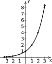
We make a table of function values, plot enough points until we are more or less confident with the shape of the curve, and connect the dots in a pleasing fashion.
Figure 7.1
A few remarks about the graph of are in order. As and takes on values like or , the function takes on values like or .
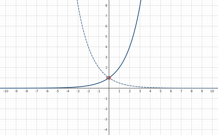
Interactive figureThe base b decides everything: y = b^x and its mirror y = (1/b)^xDrag the Base b slider from 0.25 to 4.
XYZ Graph · viewer build 5edf91b
Two exponential curves share one slider: the solid curve is y = b^x and the dashed one is y = (1/b)^x, its reflection across the y-axis. Both pass through the marked point (0, 1) no matter what b is, both stay above the x-axis, and both hug the axis on one side while racing away on the other. Drag b above 1 and the solid curve rises to the right (growth); drag it below 1 and the roles swap; at b = 1 both collapse onto the horizontal line y = 1.
In other words, as , That is, as , , so . This produces the -axis, as a horizontal asymptote to the graph as .
On the flip side, as , we find , , and so on, thus .
We note that by `connecting the dots in a pleasing fashion,' we are implicitly using the fact that is not only defined for all real numbers,1 but is also continuous. Moreover, we are assuming is increasing: that is, if , then . While these facts are true, the proofs of these properties are best left to Calculus. For us, we assume these properties in order to state the domain of is , the range of is and, since is increasing, is one-to-one, hence invertible.
Suppose we wish to study the family of functions . Which bases make sense to study? We find that we run into difficulty if . For example, if , then the function has trouble, for instance, at since is not a real number. In general, if is any rational number with an even denominator,2 then is not defined, so we must restrict our attention to bases .
What about ? The function is undefined for because we cannot divide by and is an indeterminate form. For , so the function is the same as the function , . Since we know everything about this function, we ignore this case.
The only other base we exclude is , since the function for all real numbers , since, once again, a function we have already studied. We are now ready for our definition of exponential functions.
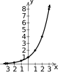
We leave it to the reader to verify3 that if , then the exponential function will share the same basic shape and characteristics as .
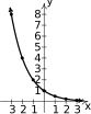
What if ? Consider . We could certainly build a table of values and connect the points, or we could take a step back and note that , where . Per Section 5.4, the graph of is obtained from the graph of by reflecting it across the -axis.
Figure 7.2
Figure 7.3
We see that the domain and range of match that of , namely and , respectively. Like , is also one-to-one. Whereas is always increasing, is always decreasing. As a result, as , and on the flip side, . (More specifically, , .) It shouldn't be too surprising that for all choices of the base , the graph of behaves similarly to the graph of .
We summarize the basic properties of exponential functions in the following theorem.
Exponential functions also inherit the basic properties of exponents from Theorem 4.3. We formalize these below and use them as needed in the coming examples.
In addition to base which is important to computer scientists,5 two other bases are used more often than not in scientific and economic circles. The first is base . Base is called the `common base' and is important in the study of intensity (sound intensity, earthquake intensity, acidity, etc.)
The second base is an irrational number, . Like or , the decimal expansion of neither terminates nor repeats, so we represent this number by the letter `.' A decimal approximation of is , so the function is an increasing exponential function.
The number is called the `natural base' for lots of reasons, one of which is that it `naturally' arises in the study of growth functions in Calculus. We will more formally discuss the origins of in Section 7.6.
It is time for an example.
Our next example showcases an important application of exponential functions: economic depreciation.
Some remarks about Example 7.1.2 are in order. First the function in the previous example is called a `decay curve'. Increasing exponential functions are used to model `growth curves' and we shall see several different examples of those in Section 7.6.
Second, as seen in numbers and, . That is to say, the function has a constant unit multiplier, in this case, because to obtain the function value , we multiply the function value by . It is not coincidence that the multiplier here is the base of the exponential, .
Indeed, exponential functions of the form have a constant unit multiplier, . To see this, note
Hence . This will prove useful to us in Section 7.6 when making decisions about whether or not a data set represents exponential growth or decay.
More generally, one can show (see Exercise ) for any real number that . That is, to obtain from , we multiply by factors of the constant unit multiplier, . This is at the heart of what it means to be an exponential function.
If this discussion seems familiar, it should. For linear functions, , we can obtain the slope by computing . To see this, note so that . In this way, we see that the slope is the constant unit addend in that in order to obtain , we add
to the function value .
This notion is solidified in the point-slope form of a linear function, Equation 1.1. For for any real numbers and , we have . If we let , we get . In other words, to obtain from , we add
times .
Taking inspiration from linear functions, we define the `point-base' form of an exponential function below.
Just as the point-slope form of a linear function is helpful in building linear models, the point-base form of an exponential function will prove useful in building exponential models.
Next, while we saw in Example 7.1.2 number, exponential functions, unlike linear functions, do not have a constant rate of change. However, in numbers and, we see that in some cases, they do have a constant relative rate of change. We define this notion below.
For exponential functions of the form , we compute the relative rate of change over the interval and find it is constant:
where we are using the fact that .
One way to interpret this result is when comparing to , the exponential function grows (if ) or decays (if ) by . In our example, so and, as we saw, the relative rate of change from to was , meaning the value of the car over the course of one year depreciates by .
We close this section with another important application of exponential functions, Newton's Law of Cooling.
Exercises
In Exercises -, sketch the graph of by starting with the graph of and using transformations. Track at least three points of your choice and the horizontal asymptote through the transformations. State the domain and range of .
,
,
,
,
,
,
,
,
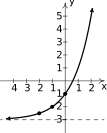
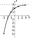
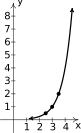
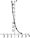
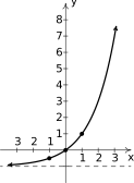
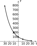
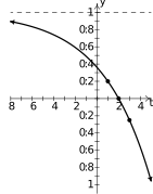
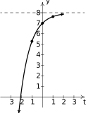
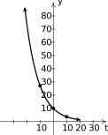
In Exercises, -, the graph of an exponential function is given. Find a formula for the function in the form .
Points: , , , Asymptote: .
Figure 7.16
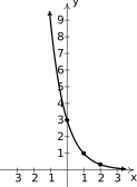
Points: , , , Asymptote: .
Figure 7.17
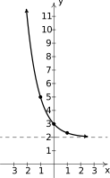
Points: , , , Asymptote: .
Figure 7.18
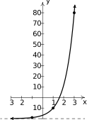
Points: , , , Asymptote: .
Figure 7.19
Find a formula for each graph in Exercises - of the form . Did you change your solution methodology? What is the relationship between your answers for and for each graph?
In Example 7.1.1 number, we obtained the solution as one formula for the given graph by making a simplifying assumption that . This exercises explores if there are any other solutions for different choices of .
Show also fits the data for the given graph, and use properties of exponents to show . (Use the fact that …)
With help from your classmates, find solutions to Example 7.1.1 number using , and . Show all your solutions can be rewritten as: .
Using properties of exponents and the fact that the range of is , show that any function of the form for can be rewritten as . Relabeling, this means every function of the form with four parameters (, , , and ) can be rewritten as , a formula with just three parameters: , , and . Conclude that every solution to Example 7.1.1 number reduces to .
In Exercises -, write the given function as a nontrivial decomposition of functions as directed.
For , find functions and so that .
For , find functions and so that .
For , find functions and so that .
For , find functions and so .
For , find functions and so that .
For , find functions and so .
The amount of money in a savings account, , in dollars, years after an initial investment is made is given by: , for .
Find and interpret , , and .
Find and interpret the relative rate of change of over the intervals , , .
Find, simplify, and interpret the relative rate of change of over the . Assume .
Use a graphing utility to estimate how long until the savings account is worth . Round your answer to the nearest year.
Based on census data,11 the population of Lake County, Ohio, in 2010 was 230,041 and in 2015, the population was 229,437.
Show the percentage change in the population from 2010 to 2015 is approximately .
If this percentage change remains constant, predict the population of Lake County in 2020.
Assuming this percentage change per five years remains constant, find an expression for the population of Lake County where is the number of five year intervals after 2010. (So corresponds to 2010, corresponds to , corresponds to , etc.)
HINT: Definitions 7.2 and 7.3 and ensuing discussion on that page is useful here.
Use your answer to to predict the population of Lake County in the year 2017.
Let represent the population of Lake County years after 2010 where the we approximate the percentage change in population per year as . Find a formula for and compare your predictions with to those given by . In particular, what population does each model give for the year 2050? Discuss any discrepancies with your classmates.
Show that the average rate of change of a function over the interval is average of the average rates of change of the function over the intervals and . Can the same be said for the average rate of change of the function over and the average of the average rates of change over , , and ? Generalize.
If where , , show .
Which is larger: or ? How do you know? Can you find a proof that doesn't use technology?
Use properties of exponential functions to show that if , then
Numerically and graphically investigate the limit:
.
Use parts and to show to your surprise and delight that the derivative of is ….
Write the equations of the tangent lines to at the following points:
Answers
Domain of : Range of : Points: , , Asymptote:
Figure 7.20
Domain of : Range of : Points: , , Asymptote:
Figure 7.21
Domain of : Range of : Points: , , Asymptote:
Figure 7.22
Domain of : Range of : Points: , , Asymptote:
Figure 7.23
Domain of : Range of : Points: , , Asymptote:
Figure 7.24
Domain of : Range of : Points: , , Asymptote:
Figure 7.25
Domain of : Range of : Points: , , Asymptote:
Figure 7.26
Domain of : Range of : Points:
, Asymptote:
Figure 7.27
Since , one way to obtain the formulas for is to use properties of exponents. For example, . In order, the formulas for are:
, so the principal is . , so after year, there is in the savings account. , so after years, there is in the savings account.
The relative rate of change of over the intervals and is which means the savings account is growing by each year for those two years. Over the interval , the relative rate of change is meaning the account has grown by over the course of the first two years. Note this is greater than the sum of the two rates . This is due to the `compounding effect' and will be discussed in greater detail in Section 7.6.
The relative rate of change of over the is . This means over the course of one year, the savings account grows by .
Graphing and , we find they intersect when so it takes approximately years for the savings account to grow to in value.
.
Since 2020 is five years after 2015, we expect the population to decrease by of 229437, or approximately 603 people. Hence, we approximate the population in 2020 as 228834.
, .
Since 2017 is 7 years after 2010, we set and find . So the population is approximately 229, 194 in 2017.
, . Since 2050 is 40 years after 2010, using the model , we divide and find . On the other hand, . This is more than roundoff error. There is a compounding effect which makes the functions and different. 13
Adapted from Precalculus with Integrated Calculus, edition 4i, by Carl Stitz and Jeff Zeager (stitz-zeager.com), licensed under CC BY-NC-SA 3.0. Changes were made: reformatted as an accessible XYZ web edition. License: CC-BY-NC-SA-3.0.
These eBooks are a prerelease and are not yet certified conformant with WCAG 2.1 AA or any other accessibility standard. Every page is built against an automated accessibility gate, and our target for the published editions is WCAG 2.2 Level AA. If something is unusable, please tell us.