7.3 Properties of Logarithms

In Section 7.2, we introduced the logarithmic functions as inverses of exponential functions and discussed a few of their functional properties from that perspective. In this section, we explore the algebraic properties of logarithms. Historically, these have played a huge role in the scientific development of our society since, among other things, they were used to develop analog computing devices called slide rules which enabled scientists and engineers to perform accurate calculations leading to such things as space travel and the moon landing.

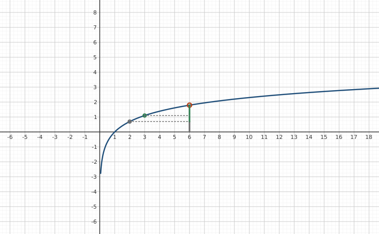
As we shall see shortly, logs inherit analogs of all of the properties of exponents you learned in Elementary and Intermediate Algebra. We first extract two properties from Theorem 7.3 to remind us of the definition of a logarithm as the inverse of an exponential function.

Theorem

(Inverse Properties of Exponential and Logarithmic Functions)

Let $b greater than 0$ , $b not equal to 1$ .

$b^{a} = c$ if and only if $\log_{b} (c) = a$ . That is, $\log_{b} (c)$ is the exponent you put on $b$ to obtain $c$ .
$\log_{b} (b^{x}) = x$ for all $x$ and $b^{\log_{b} (x)} = x$ for all $x greater than 0$

Next, we spell out what it means for exponential and logarithmic functions to be one-to-one.

Theorem

(One-to-one Properties of Exponential and Logarithmic Functions)

Let $f (x) = b^{x}$ and $g (x) = \log_{b} (x)$ where $b greater than 0$ , $b not equal to 1$ . Then $f$ and $g$ are one-to-one and

$b^{u} = b^{w}$ if and only if $u = w$ for all real numbers $u$ and $w$ .
$\log_{b} (u) = \log_{b} (w)$ if and only if $u = w$ for all real numbers $u greater than 0$ , $w greater than 0$ .

Next, we re-state Theorem 7.2 for reference below.

Theorem

(Algebraic Properties of Exponential Functions) Let $f (x) = b^{x}$ be an exponential function ( $b greater than 0$ , $b not equal to 1$ ) and let $u$ and $w$ be real numbers.

Product Rule: $f (u + w) = f (u) f (w)$ . In other words, $b^{u + w} = b^{u} b^{w}$
Quotient Rule: $f (u - w) = \frac{f (u)}{f (w)}$ . In other words, $b^{u - w} = \frac{b^{u}}{b^{w}}$
Power Rule: ${(f (u))}^{w} = f (u w)$ . In other words, ${(b^{u})}^{w} = b^{u w}$

To each of these properties of listed in Theorem 7.2, there corresponds an analogous property of logarithmic functions. We list these below in our next theorem.

Theorem

(Algebraic Properties of Logarithmic Functions) Let $g (x) = \log_{b} (x)$ be a logarithmic function ( $b greater than 0$ , $b not equal to 1$ ) and let $u greater than 0$ and $w greater than 0$ be real numbers.

Product Rule: $g (u w) = g (u) + g (w)$ . In other words, $\log_{b} (u w) = \log_{b} (u) + \log_{b} (w)$
Quotient Rule: $g (\frac{u}{w}) = g (u) - g (w)$ . In other words, $\log_{b} (\frac{u}{w}) = \log_{b} (u) - \log_{b} (w)$
Power Rule: $g (u^{w}) = w g (u)$ . In other words, $\log_{b} (u^{w}) = w \log_{b} (u)$

There are a couple of different ways to understand why Theorem 7.7 is true. For instance, consider the product rule: $\log_{b} (u w) = \log_{b} (u) + \log_{b} (w)$ .

Let $a = \log_{b} (u w)$ , $c = \log_{b} (u)$ , and $d = \log_{b} (w)$ . Then, by definition, $b^{a} = u w$ , $b^{c} = u$ and $b^{d} = w$ . Hence, $b^{a} = u w = b^{c} b^{d} = b^{c + d}$ , so that $b^{a} = b^{c + d}$ .

By the one-to-one property of $b^{x}$ , $b^{a} = b^{c + d}$ gives $a = c + d$ . In other words, $\log_{b} (u w) = \log_{b} (u) + \log_{b} (w)$ . The remaining properties are proved similarly.

From a purely functional approach, we can see the properties in Theorem 7.7 as an example of how inverse functions interchange the roles of inputs in outputs.

For instance, the Product Rule for exponential functions given in Theorem 7.2, $f (u + w) = f (u) f (w)$ , says that adding inputs results in multiplying outputs.

Hence, whatever $f^{- 1}$ is, it must take the products of outputs from $f$ and return them to the sum of their respective inputs. Since the outputs from $f$ are the inputs to $f^{- 1}$ and vice-versa, we have that that $f^{- 1}$ must take products of its inputs to the sum of their respective outputs. This is precisely one way to interpret the Product Rule for Logarithmic functions: $g (u w) = g (u) + g (w)$ .

The reader is encouraged to view the remaining properties listed in Theorem 7.7 similarly.

The following examples help build familiarity with these properties. In our first example, we are asked to `expand' the logarithms. This means that we read the properties in Theorem 7.7 from left to right and rewrite products inside the log as sums outside the log, quotients inside the log as differences outside the log, and powers inside the log as factors outside the log.¹

Example 1

Expand the following using the properties of logarithms and simplify. Assume when necessary that all quantities represent positive real numbers.

$\log_{2} (\frac{8}{x})$
$log sub 0.1 ⁡ open parenthesis 10 ⁢ x squared close parenthesis$
$\ln {(\frac{3}{e t})}^{2}$
$\log \sqrt[3]{\frac{100 x^{2}}{y z^{5}}}$
$log sub 117 ⁡ open parenthesis x squared minus 4 close parenthesis$

To expand $\log_{2} (\frac{8}{x})$ , we use the Quotient Rule identifying $u equals 8$ and $w = x$ and simplify.
$\begin{matrix} \log_{2} (\frac{8}{x}) & = & \log_{2} (8) - \log_{2} (x) & Quotient Rule \\ = & 3 - \log_{2} (x) & Since 2^{3} = 8 \\ = & - \log_{2} (x) + 3 \end{matrix}$
In the expression $log sub 0.1 ⁡ open parenthesis 10 ⁢ x squared close parenthesis$ , we have a power (the $x^{2}$ ) and a product, and the question becomes which property, Power Rule or Product Rule to use first.
In order to use the Power Rule, the entire quantity inside the log must be raised to the same exponent. Since the exponent $2$ applies only to the $x$ , we first apply the Product Rule with $u equals 10$ and $w = x^{2}$ . Once the $x^{2}$ is by itself inside the log, we apply the Power Rule with $u = x$ and $w equals 2$ .
$\begin{matrix} \log_{0.1} (10 x^{2}) & = & \log_{0.1} (10) + \log_{0.1} (x^{2}) & Product Rule \\ = & \log_{0.1} (10) + 2 \log_{0.1} (x) & Power Rule \\ = & - 1 + 2 \log_{0.1} (x) & Since {(0.1)}^{- 1} = 10 \\ = & 2 \log_{0.1} (x) - 1 \end{matrix}$
We have a power, quotient and product occurring in $\ln {(\frac{3}{e t})}^{2}$ . Since the exponent $2$ applies to the entire quantity inside the logarithm, we begin with the Power Rule with $u = \frac{3}{e t}$ and $w equals 2$ .
Next, we see the Quotient Rule is applicable, with $u equals 3$ and $w = e t$ , so we replace $\ln (\frac{3}{e t})$ with the quantity $ln ⁡ open parenthesis 3 close parenthesis minus ln ⁡ open parenthesis e ⁢ t close parenthesis$ .
Since $\ln (\frac{3}{e t})$ is being multiplied by $2$ , the entire quantity $ln ⁡ open parenthesis 3 close parenthesis minus ln ⁡ open parenthesis e ⁢ t close parenthesis$ is multiplied by $2$ .
Finally, we apply the Product Rule with $u = e$ and $w = x$ , and replace $\ln (e t)$ with the quantity $\ln (e) + \ln (t)$ , and simplify, keeping in mind that the natural log is log base $e$ .
$\begin{matrix} \ln {(\frac{3}{e t})}^{2} & = & 2 \ln (\frac{3}{e t}) & Power Rule \\ = & 2 [\ln (3) - \ln (e t)] & Quotient Rule \\ = & 2 \ln (3) - 2 \ln (e t) \\ = & 2 \ln (3) - 2 [\ln (e) + \ln (t)] & Product Rule \\ = & 2 \ln (3) - 2 \ln (e) - 2 \ln (t) \\ = & 2 \ln (3) - 2 - 2 \ln (t) & Since e^{1} = e \\ = & - 2 \ln (t) + 2 \ln (3) - 2 \end{matrix}$
In Theorem 7.7, there is no mention of how to deal with radicals. However, thinking back to Definition A.9, we can rewrite the cube root as a $\frac{1}{3}$ exponent. We begin by using the Power Rule², and we keep in mind that the common log is log base $10$ .
$\begin{matrix} \log \sqrt[3]{\frac{100 x^{2}}{y z^{5}}} & = & \log {(\frac{100 x^{2}}{y z^{5}})}^{1 / 3} \\ = & \frac{1}{3} \log (\frac{100 x^{2}}{y z^{5}}) & Power Rule \\ = & \frac{1}{3} [\log (100 x^{2}) - \log (y z^{5})] & Quotient Rule \\ = & \frac{1}{3} \log (100 x^{2}) - \frac{1}{3} \log (y z^{5}) \\ = & \frac{1}{3} [\log (100) + \log (x^{2})] - \frac{1}{3} [\log (y) + \log (z^{5})] & Product Rule \\ = & \frac{1}{3} \log (100) + \frac{1}{3} \log (x^{2}) - \frac{1}{3} \log (y) - \frac{1}{3} \log (z^{5}) \\ = & \frac{1}{3} \log (100) + \frac{2}{3} \log (x) - \frac{1}{3} \log (y) - \frac{5}{3} \log (z) & Power Rule \\ = & \frac{2}{3} + \frac{2}{3} \log (x) - \frac{1}{3} \log (y) - \frac{5}{3} \log (z) & Since 10^{2} = 100 \\ = & \frac{2}{3} \log (x) - \frac{1}{3} \log (y) - \frac{5}{3} \log (z) + \frac{2}{3} \end{matrix}$
At first it seems as if we have no means of simplifying $log sub 117 ⁡ open parenthesis x squared minus 4 close parenthesis$ , since none of the properties of logs addresses the issue of expanding a difference inside the logarithm. However, we may factor $x^{2} - 4 = (x + 2) (x - 2)$ thereby introducing a product which gives us license to use the Product Rule. Assuming both $x plus 2 greater than 0$ and $x minus 2 greater than 0$ , that is, $x greater than 2$ we expand as follows.
$\begin{matrix} \log_{117} (x^{2} - 4) & = & \log_{117} [(x + 2) (x - 2)] & Factor \\ = & \log_{117} (x + 2) + \log_{117} (x - 2) & Product Rule \end{matrix}$

A couple of remarks about Example 7.3.1 are in order. First, if we take a step back and look at each problem in the foregoing example, a general rule of thumb to determine which log property to apply first when faced with a multi-step problem is to apply the logarithm properties in the `reverse order of operations.'

For example, if we were to substitute a number for $x$ into the expression $log sub 0.1 ⁡ open parenthesis 10 ⁢ x squared close parenthesis$ , we would first square the $x$ , then multiply by $10$ . The last step is the multiplication, which tells us the first log property to apply is the Product Rule. The last property of logarithm to apply would the be the power rule applied to $log sub 0.1 ⁡ open parenthesis x squared close parenthesis$ .

Second, the equivalence $\log_{117} (x^{2} - 4) = \log_{117} (x + 2) + \log_{117} (x - 2)$ is valid only if $x greater than 2$ . Indeed, the functions $f (x) = \log_{117} (x^{2} - 4)$ and $g (x) = \log_{117} (x + 2) + \log_{117} (x - 2)$ have different domains, and, hence, are different functions.³ In general, when using log properties to expand a logarithm, we may very well be restricting the domain as we do so.

One last comment before we move to reassembling logs from their various bits and pieces. The authors are well aware of the propensity for some students to become overexcited and invent their own properties of logs like $\log_{117} (x^{2} - 4) = \log_{117} (x^{2}) - \log_{117} (4)$ , which simply isn't true, in general. The unwritten⁴ property of logarithms is that if it isn't written in a textbook, it probably isn't true.

Example 2

Use the properties of logarithms to write the following as a single logarithm.

$\log_{3} (x - 1) - \log_{3} (x + 1)$
$\log (x) + 2 \log (y) - \log (z)$
$4 ⁢ log sub 2 ⁡ open parenthesis x close parenthesis plus 3$
$- \ln (t) - \frac{1}{2}$

Whereas in Example 7.3.1 we read the properties in Theorem 7.7 from left to right to expand logarithms, in this example we read them from right to left.

The difference of logarithms requires the Quotient Rule: $\log_{3} (x - 1) - \log_{3} (x + 1) = \log_{3} (\frac{x - 1}{x + 1})$ .
In the expression, $\log (x) + 2 \log (y) - \log (z)$ , we have both a sum and difference of logarithms.
Before we use the product rule to combine $log ⁡ open parenthesis x close parenthesis plus 2 ⁢ log ⁡ open parenthesis y close parenthesis$ , we note that we need to apply the Power Rule to rewrite the coefficient $2$ as the power on $y$ . We then apply the Product and Quotient Rules as we move from left to right.
$\begin{matrix} \log (x) + 2 \log (y) - \log (z) & = & \log (x) + \log (y^{2}) - \log (z) & Power Rule \\ = & \log (x y^{2}) - \log (z) & Product Rule \\ = & \log (\frac{x y^{2}}{z}) & Quotient Rule \end{matrix}$
We begin rewriting $4 ⁢ log sub 2 ⁡ open parenthesis x close parenthesis plus 3$ by applying the Power Rule: $4 \log_{2} (x) = \log_{2} (x^{4})$ .
In order to continue, we need to rewrite $3$ as a logarithm base $2$ . From Theorem 7.4, we know $3 equals log sub 2 ⁡ open parenthesis 2 cubed close parenthesis$ . Rewriting $3$ this way paves the way to use the Product Rule.
$\begin{matrix} 4 \log_{2} (x) + 3 & = & \log_{2} (x^{4}) + 3 & Power Rule \\ = & \log_{2} (x^{4}) + \log_{2} (2^{3}) & Since 3 = \log_{2} (2^{3}) \\ = & \log_{2} (x^{4}) + \log_{2} (8) \\ = & \log_{2} (8 x^{4}) & Product Rule \end{matrix}$
To get started with $- \ln (t) - \frac{1}{2}$ , we rewrite $- \ln (t)$ as $open parenthesis minus 1 close parenthesis ⁢ ln ⁡ open parenthesis t close parenthesis$ . We can then use the Power Rule to obtain $(- 1) \ln (t) = \ln (t^{- 1})$ .
As in the previous problem, in order to continue, we need to rewrite $\frac{1}{2}$ as a natural logarithm. Theorem 7.4 gives us $\frac{1}{2} = \ln (e^{1 / 2}) = \ln (\sqrt{e})$ . Hence,
$\begin{matrix} - \ln (t) - \frac{1}{2} & = & (- 1) \ln (t) - \frac{1}{2} \\ = & \ln (t^{- 1}) - \frac{1}{2} & Power Rule \\ = & \ln (t^{- 1}) - \ln (e^{1 / 2}) & Since \frac{1}{2} = \ln (e^{1 / 2}) \\ = & \ln (t^{- 1}) - \ln (\sqrt{e}) \\ = & \ln (\frac{t^{- 1}}{\sqrt{e}}) & Quotient Rule \\ = & \ln (\frac{1}{t \sqrt{e}}) \end{matrix}$

As we would expect, the rule of thumb for re-assembling logarithms is the opposite of what it was for dismantling them. That is, to rewrite an expression as a single logarithm, we apply log properties following the usual order of operations: first, rewrite coefficients of logs as powers using the Power Rule, then rewrite addition and subtraction using the Product and Quotient Rules, respectively, as written from left to right.

Additionally, we find that using log properties in this fashion can increase the domain of the expression. For example, we leave it to the reader to verify the domain of $f (x) = \log_{3} (x - 1) - \log_{3} (x + 1)$ is $open parenthesis 1, ∞ close parenthesis$ but the domain of $g (x) = \log_{3} (\frac{x - 1}{x + 1})$ is $(- \infty, - 1) \cup (1, \infty)$ . We'll need to keep this in mind in Section 7.5 since such manipulations can result in extraneous solutions.

The two logarithm buttons commonly found on calculators are the `LOG' and `LN' buttons which correspond to the common and natural logs, respectively. Suppose we wanted an approximation to $log sub 2 ⁡ open parenthesis 7 close parenthesis$ . The answer should be a little less than $3$ , (Can you explain why?) but how do we coerce the calculator into telling us a more accurate answer? We need the following theorem.

Theorem

(Change of Base Formulas) Let $a, b greater than 0$ , $a, b not equal to 1$ .

$a^{x} = b^{x \log_{b} (a)}$ for all real numbers $x$ .
$\log_{a} (x) = \frac{\log_{b} (x)}{\log_{b} (a)}$ for all real numbers $x greater than 0$ .

To prove these formulas, consider $b^{x \log_{b} (a)}$ . Using the Power Rule, we can rewrite $x \log_{b} (a)$ as $\log_{b} (a^{x})$ . Following this with the Inverse Properties in Theorem 7.4, we get

$b^{x \log_{b} (a)} = b^{\log_{b} (a^{x})} = a^{x} .$

To verify the logarithmic form of the property, we use the Power Rule and an Inverse Property to get:

$\log_{a} (x) \cdot \log_{b} (a) = \log_{b} (a^{\log_{a} (x)}) = \log_{b} (x) .$

We get the result by dividing both sides of the equation $\log_{a} (x) \cdot \log_{b} (a) = \log_{b} (x)$ by $\log_{b} (a)$ .

Of course, the authors can't help but point out the inverse relationship between these two change of base formulas. To change the base of an exponential expression, we multiply the input by the factor $\log_{b} (a)$ . To change the base of a logarithmic expression, we divide the output by the factor $\log_{b} (a)$ .

While, in the grand scheme of things, both change of base formulas are really saying the same thing, the logarithmic form is the one usually encountered in Algebra while the exponential form isn't usually introduced until Calculus.

Example 3

Use an appropriate change of base formula to convert the following expressions to ones with the indicated base. Verify your answers using a graphing utility, as appropriate.

$3 squared$ to base $10$
$2 to the power x$ to base $e$
$log sub 4 ⁡ open parenthesis 5 close parenthesis$ to base $e$
$\ln (x)$ to base $10$

We apply the Change of Base formula with $a equals 3$ and $b equals 10$ to obtain $3^{2} = 10^{2 \log (3)}$ . Typing the latter into a graphing utility produces an answer of $9$ as seen below.
Here, $a equals 2$ and $b = e$ so we have $2^{x} = e^{x \ln (2)}$ . Using a graphing utility, we find the graphs of $f (x) = 2^{x}$ and $g (x) = e^{x \ln (2)}$ appear to overlap perfectly.
Figure 7.61
Applying the change of base with $a equals 4$ and $b = e$ leads us to write $\log_{4} (5) = \frac{\ln (5)}{\ln (4)}$ . Evaluating this gives the numerical approximation $\frac{\ln (5)}{\ln (4)} \approx 1.16$ .
To check our answer we know that, by definition, $log sub 4 ⁡ open parenthesis 5 close parenthesis$ is the exponent we put on $4$ to get $5$ , so a number a little larger than $1$ seems reasonable.
Taking this one step further, we use a graphing utility and find $4^{\frac{\ln (5)}{\ln (4)}} = 5$ , which means if the machine is lying to us about the first answer it gave us, at least it is being consistent.
We write $\ln (x) = \log_{e} (x) = \frac{\log (x)}{\log (e)}$ . We graph both $f (x) = \ln (x)$ and $g (x) = \frac{\log (x)}{\log (e)}$ and find both graphs appear to be identical.
Figure 7.62

What Theorem 7.8 really tells us is that all exponential and logarithmic functions are just scalings of one another. Not only does this explain why their graphs have similar shapes, but it also tells us that we could do all of mathematics with a single base, be it $10$ , $0.42$ , $π$ , or $117$ .

As mentioned in Section 7.1, the `natural' base, base $e$ , features prominently in mathematical applications as we'll see in Section 7.6. Hence, we conclude this section by specifying Theorem 7.8 to this case.

Theorem

Conversion to the Natural Base: Suppose $b greater than 0$ , $b not equal to 1$ . Then

$b^{x} = e^{x \ln (b)}$ for all real numbers $x$ .
$\log_{b} (x) = \frac{\ln (x)}{\ln (b)}$ for all real numbers $x greater than 0$ .

Exercises

In Exercises -, expand the given logarithm and simplify. Assume when necessary that all quantities represent positive real numbers.

$\ln (x^{3} y^{2})$
$\log_{2} (\frac{128}{x^{2} + 4})$
$\log_{5} {(\frac{z}{25})}^{3}$
$\log (1.23 \times 10^{37})$
$\ln (\frac{\sqrt{z}}{x y})$
$log sub 5 ⁡ open parenthesis x squared minus 25 close parenthesis$
$log sub the square root of 2 ⁡ open parenthesis 4 ⁢ x cubed close parenthesis$
$\log_{\frac{1}{3}} (9 x (y^{3} - 8))$
$log ⁡ open parenthesis 1000 ⁢ x cubed ⁢ y to the power 5 close parenthesis$
$\log_{3} (\frac{x^{2}}{81 y^{4}})$
$\ln (\sqrt[4]{\frac{x y}{e z}})$
$\log_{6} {(\frac{216}{x^{3} y})}^{4}$
$\log (\frac{100 x \sqrt{y}}{\sqrt[3]{10}})$
$\log_{\frac{1}{2}} (\frac{4 \sqrt[3]{x^{2}}}{y \sqrt{z}})$
$\ln (\frac{\sqrt[3]{x}}{10 \sqrt{y z}})$

In Exercises -, use the properties of logarithms to write the expression as a single logarithm.

$4 ⁢ ln ⁡ open parenthesis x close parenthesis plus 2 ⁢ ln ⁡ open parenthesis y close parenthesis$
$\log_{2} (x) + \log_{2} (y) - \log_{2} (z)$
$log sub 3 ⁡ open parenthesis x close parenthesis minus 2 ⁢ log sub 3 ⁡ open parenthesis y close parenthesis$
$\frac{1}{2} \log_{3} (x) - 2 \log_{3} (y) - \log_{3} (z)$
$2 \ln (x) - 3 \ln (y) - 4 \ln (z)$
$\log (x) - \frac{1}{3} \log (z) + \frac{1}{2} \log (y)$
$- \frac{1}{3} \ln (x) - \frac{1}{3} \ln (y) + \frac{1}{3} \ln (z)$
$log sub 5 ⁡ open parenthesis x close parenthesis minus 3$
$3 minus log ⁡ open parenthesis x close parenthesis$
$\log_{7} (x) + \log_{7} (x - 3) - 2$
$\ln (x) + \frac{1}{2}$
$log sub 2 ⁡ open parenthesis x close parenthesis plus log sub 4 ⁡ open parenthesis x close parenthesis$
$\log_{2} (x) + \log_{4} (x - 1)$
$\log_{2} (x) + \log_{\frac{1}{2}} (x - 1)$

In Exercises -, use the appropriate change of base formula to convert the given expression to an expression with the indicated base.

$7^{x - 1}$ to base $e$
$log sub 3 ⁡ open parenthesis x plus 2 close parenthesis$ to base 10
${(\frac{2}{3})}^{x}$ to base $e$
$log ⁡ open parenthesis x squared plus 1 close parenthesis$ to base $e$

In Exercises -, use the appropriate change of base formula to approximate the logarithm.

$log sub 3 ⁡ open parenthesis 12 close parenthesis$
$log sub 5 ⁡ open parenthesis 80 close parenthesis$
$log sub 6 ⁡ open parenthesis 72 close parenthesis$
$\log_{4} (\frac{1}{10})$
$\log_{\frac{3}{5}} (1000)$
$\log_{\frac{2}{3}} (50)$
In Example 7.2.1 number in Section 7.2, we obtained the solution $F (x) = \log_{2} (- x + 4) - 3$ as one formula for the given graph by making a simplifying assumption that $b = - 1$ . This exercises explores if there are any other solutions for different choices of $b$ .
1. Show $G (x) = \log_{2} (- 2 x + 8) - 4$ also fits the data for the given graph.
2. Use properties of logarithms to show $G (x) = \log_{2} (- 2 x + 8) - 4 = \log_{2} (- x + 4) - 3 = F (x)$ .
3. With help from your classmates, find solutions to Example 7.2.1 number in Section 7.2 by assuming $b = - 4$ and $b = - 8$ . In each case, use properties of logarithms to show the solutions reduce to $F (x) = \log_{2} (- x + 4) - 3$ .
4. Using properties of logarithms and the fact that the range of $log sub 2 ⁡ open parenthesis x close parenthesis$ is all real numbers, show that any function of the form $f (x) = a \log_{2} (b x - h) + k$ where $a not equal to 0$ can be rewritten as:
  $f (x) = a (\log_{2} (b x - h) + \frac{k}{a}) = a (\log_{2} (b x - h) + \log_{2} (p)) = a \log_{2} (p (b x - h)) = a \log_{2} (p b x - p h),$
  where $\frac{k}{a} = \log_{2} (p)$ for some positive real number $p$ . Relabeling, we get every function of the form $f (x) = a \log_{2} (b x - h) + k$ with four parameters ( $a$ , $b$ , $h$ , and $k$ ) can be rewritten as $f (x) = a \log_{2} (B x - H)$ , a formula with just three parameters: $a$ , $B$ , and $H$ .
  Show every solution to Example 7.2.1 number in Section 7.2 can be written in the form $f (x) = \log_{2} (- \frac{1}{8} x + \frac{1}{2})$ and that, in particular, $F (x) = \log_{2} (- x + 4) - 3 = \log_{2} (- \frac{1}{8} x + \frac{1}{2}) = f (x)$ . Hence, there is really just one solution to Example 7.2.1 number in Section 7.2.
The Henderson-Hasselbalch Equation: Suppose $H A$ represents a weak acid. Then we have a reversible chemical reaction
$H A ⇌ H^{+} + A^{-} .$
The acid disassociation constant, $K_{a}$ , is given by
$K_{a} = \frac{[H^{+}] [A^{-}]}{[H A]} = [H^{+}] \frac{[A^{-}]}{[H A]},$
where the square brackets denote the concentrations just as they did in Exercise in Section 7.2. The symbol p $K_{a}$ is defined similarly to pH in that p $K_{a} = - \log (K_{a})$ . Using the definition of pH from Exercise and the properties of logarithms, derive the Henderson-Hasselbalch Equation:
$pH = p K_{a} + \log \frac{[A^{-}]}{[H A]}$
Compare and contrast the graphs of $y = \ln (x^{2})$ and $y equals 2 ⁢ ln ⁡ open parenthesis x close parenthesis$ .
Prove the Quotient Rule and Power Rule for Logarithms.
Give numerical examples to show that, in general,
1. $\log_{b} (x + y) \neq \log_{b} (x) + \log_{b} (y)$
2. $\log_{b} (x - y) \neq \log_{b} (x) - \log_{b} (y)$
1. $\log_{b} (\frac{x}{y}) \neq \frac{\log_{b} (x)}{\log_{b} (y)}$
Research the history of logarithms including the origin of the word `logarithm' itself. Why is the abbreviation of natural log `ln' and not `nl'?
There is a scene in the movie `Apollo 13' in which several people at Mission Control use slide rules to verify a computation. Was that scene accurate? Look for other pop culture references to logarithms and slide rules.
1. Use properties of logarithm functions to show that if $f (x) = \ln (x)$ , then
  $f^{'} (x) = lim_{h \to 0} \frac{f (x + h) - f (x)}{h} = lim_{h \to 0} \frac{\ln (1 + \frac{h}{x})}{h}$
2. Numerically and graphically investigate the limit: $lim h → 0$ $\frac{\ln (1 + \frac{h}{x})}{h}$ for various positive numbers $x$ to convince yourself that $lim h → 0$ $\frac{\ln (1 + \frac{h}{x})}{h} = \frac{1}{x}$
3. Use parts and to show to show that the derivative of $\ln (x)$ is … $\frac{1}{x}$ .
4. Write the equations of the tangent lines to $y = \ln (x)$ at the following points. Check your answers graphically. Compare your answers the tangent lines at the corresponding points in Exercise in Section 7.1.
  1. $open parenthesis 1, 0 close parenthesis$
  2. $open parenthesis e, 1 close parenthesis$
  3. $(e^{- 1}, - 1)$

Answers

$3 ⁢ ln ⁡ open parenthesis x close parenthesis plus 2 ⁢ ln ⁡ open parenthesis y close parenthesis$
$7 - \log_{2} (x^{2} + 4)$
$3 ⁢ log sub 5 ⁡ open parenthesis z close parenthesis minus 6$
$log ⁡ open parenthesis 1.23 close parenthesis plus 37$
$\frac{1}{2} \ln (z) - \ln (x) - \ln (y)$
$\log_{5} (x - 5) + \log_{5} (x + 5)$
$3 \log_{\sqrt{2}} (x) + 4$
$- 2 + \log_{\frac{1}{3}} (x) + \log_{\frac{1}{3}} (y - 2) + \log_{\frac{1}{3}} (y^{2} + 2 y + 4)$
$3 + 3 \log (x) + 5 \log (y)$
$2 \log_{3} (x) - 4 - 4 \log_{3} (y)$
$\frac{1}{4} \ln (x) + \frac{1}{4} \ln (y) - \frac{1}{4} - \frac{1}{4} \ln (z)$
$12 - 12 \log_{6} (x) - 4 \log_{6} (y)$
$\frac{5}{3} + \log (x) + \frac{1}{2} \log (y)$
$- 2 + \frac{2}{3} \log_{\frac{1}{2}} (x) - \log_{\frac{1}{2}} (y) - \frac{1}{2} \log_{\frac{1}{2}} (z)$
$\frac{1}{3} \ln (x) - \ln (10) - \frac{1}{2} \ln (y) - \frac{1}{2} \ln (z)$
$ln ⁡ open parenthesis x to the power 4 ⁢ y squared close parenthesis$
$\log_{2} (\frac{x y}{z})$
$\log_{3} (\frac{x}{y^{2}})$
$\log_{3} (\frac{\sqrt{x}}{y^{2} z})$
$\ln (\frac{x^{2}}{y^{3} z^{4}})$
$\log (\frac{x \sqrt{y}}{\sqrt[3]{z}})$
$\ln (\sqrt[3]{\frac{z}{x y}})$
$\log_{5} (\frac{x}{125})$
$\log (\frac{1000}{x})$
$\log_{7} (\frac{x (x - 3)}{49})$
$\ln (x \sqrt{e})$
$log sub 2 ⁡ open parenthesis x to the power 3 / 2 close parenthesis$
$\log_{2} (x \sqrt{x - 1})$
$\log_{2} (\frac{x}{x - 1})$
$7^{x - 1} = e^{(x - 1) \ln (7)}$
$\log_{3} (x + 2) = \frac{\log (x + 2)}{\log (3)}$
${(\frac{2}{3})}^{x} = e^{x \ln (\frac{2}{3})}$
$\log (x^{2} + 1) = \frac{\ln (x^{2} + 1)}{\ln (10)}$
$log sub 3 ⁡ open parenthesis 12 close parenthesis approximately equals 2.26186$
$log sub 5 ⁡ open parenthesis 80 close parenthesis approximately equals 2.72271$
$log sub 6 ⁡ open parenthesis 72 close parenthesis approximately equals 2.38685$
$\log_{4} (\frac{1}{10}) \approx - 1.66096$
$\log_{\frac{3}{5}} (1000) \approx - 13.52273$
$\log_{\frac{2}{3}} (50) \approx - 9.64824$
1. 1. $y = x - 1$
  2. $y = \frac{1}{e} x$
  3. $y = e x - 2$

Interestingly enough, it is the exact opposite process (which we will practice later) that is most useful in Algebra, the utility of expanding logarithms becomes apparent in Calculus. ↩
At this point in the text, the reader is encouraged to carefully read through each step and think of which quantity is playing the role of $u$ and which is playing the role of $w$ as we apply each property. ↩
We leave it to the reader to verify the domain of $f$ is $(- \infty, - 2) \cup (2, \infty)$ whereas the domain of $g$ is $open parenthesis 2, ∞ close parenthesis$ . ↩
The authors relish the irony involved in writing what follows. ↩

Adapted from Precalculus, Preliminary 4th Edition (integrated calculus), by Carl Stitz and Jeff Zeager (stitz-zeager.com), licensed under CC BY-NC-SA 3.0. Changes were made: reformatted as an accessible XYZ web edition. License: CC-BY-NC-SA-3.0.