7.5 Equations and Inequalities involving Logarithmic Functions

In Section 7.4 we solved equations and inequalities involving exponential functions using one of two basic strategies. We now turn our attention to equations and inequalities involving logarithmic functions, and not surprisingly, there are two basic strategies to choose from.

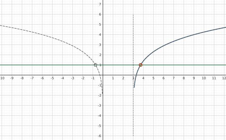
For example, per Theorem 7.5, the only solution to $log sub 2 ⁡ open parenthesis x close parenthesis equals log sub 2 ⁡ open parenthesis 5 close parenthesis$ is $x equals 5$ . Now consider $log sub 2 ⁡ open parenthesis x close parenthesis equals 3$ . To use Theorem 7.5, we need to rewrite $3$ as a logarithm base $2$ . Theorem 7.4 gives us $3 = \log_{2} (2^{3}) = \log_{2} (8)$ . Hence, $log sub 2 ⁡ open parenthesis x close parenthesis equals 3$ is equivalent to $log sub 2 ⁡ open parenthesis x close parenthesis equals log sub 2 ⁡ open parenthesis 8 close parenthesis$ so that $x equals 8$ .

A second approach to solving $log sub 2 ⁡ open parenthesis x close parenthesis equals 3$ us to apply the corresponding exponential function, $f (x) = 2^{x}$ to both sides: $2^{\log_{2} (x)} = 2^{3}$ so $x = 2^{3} = 8$ .

A third approach to solving $log sub 2 ⁡ open parenthesis x close parenthesis equals 3$ is to use Theorem 7.4 to rewrite $log sub 2 ⁡ open parenthesis x close parenthesis equals 3$ as $2 cubed equals x$ , so $x equals 8$ .

In the grand scheme of things, all three approaches we have presented to solve $log sub 2 ⁡ open parenthesis x close parenthesis equals 3$ are mathematically equivalent, so we opt to choose the last approach in our summary below.

Steps for Solving an Equation involving Logarithmic Functions

Isolate the logarithmic function.
1. If convenient, express both sides as logs with the same base and equate arguments.
2. Otherwise, rewrite the log equation as an exponential equation.

Example 1

Solve the following equations. Check your solutions graphically using a calculator.

$\log_{117} (1 - 3 x) = \log_{117} (x^{2} - 3)$
$2 - \ln (t - 3) = 1$
$\log_{6} (x + 4) + \log_{6} (3 - x) = 1$
$\log_{7} (1 - 2 t) = 1 - \log_{7} (3 - t)$
$\log_{2} (x + 3) = \log_{2} (6 - x) + 3$
$1 + 2 \log_{4} (t + 1) = 2 \log_{2} (t)$

Since we have the same base on both sides of the equation $\log_{117} (1 - 3 x) = \log_{117} (x^{2} - 3)$ , we equate the arguments (what's inside) of the logs to get $1 - 3 x = x^{2} - 3$ . Solving $x^{2} + 3 x - 4 = 0$ gives $x = - 4$ and $x equals 1$ .
To check these answers using a graphing utility, we make use of the change of base formula and graph $f (x) = \frac{\ln (1 - 3 x)}{\ln (117)}$ and $g (x) = \frac{\ln (x^{2} - 3)}{\ln (117)}$ . We see these graphs intersect only at $x = - 4$ . however.
To see what happened to the solution $x equals 1$ , we substitute it into our original equation to obtain $\log_{117} (- 2) = \log_{117} (- 2)$ . While these expressions look identical, neither is a real number,¹ which means $x equals 1$ is not in the domain of the original equation, and is not a solution.
To solve $2 - \ln (t - 3) = 1$ , we first isolate the logarithm and get $\ln (t - 3) = 1$ . Rewriting $\ln (t - 3) = 1$ as an exponential equation, we get is $e^{1} = t - 3$ , so $t = e + 3$ .
A graphing utility shows the graphs of $f (t) = 2 - \ln (t - 3)$ and $g ⁢ open parenthesis t close parenthesis equals 1$ intersect at $t \approx 5.718 \approx e + 3$ .
Figure 7.82
Figure 7.83
Checking $\log_{117} (1 - 3 x) = \log_{117} (x^{2} - 3)$
Checking $2 - \ln (t - 3) = 1$
We start solving $\log_{6} (x + 4) + \log_{6} (3 - x) = 1$ by using the Product Rule for logarithms to rewrite the equation as $\log_{6} [(x + 4) (3 - x)] = 1$ .
Rewriting as an exponential equation gives $6^{1} = (x + 4) (3 - x)$ which reduces to $x^{2} + x - 6 = 0$ . We get two solutions: $x = - 3$ and $x equals 2$ .
Using the change of base formula, we graph $y = f (x) = \frac{\ln (x + 4)}{\ln (6)} + \frac{\ln (3 - x)}{\ln (6)}$ and $y = g (x) = 1$ and we see the graphs intersect twice, at $x = - 3$ and $x equals 2$ , as required.
Taking a cue from the previous problem, we begin solving $\log_{7} (1 - 2 t) = 1 - \log_{7} (3 - t)$ by first collecting the logarithms on the same side, $\log_{7} (1 - 2 t) + \log_{7} (3 - t) = 1$ , and then using the Product Rule to get $\log_{7} [(1 - 2 t) (3 - t)] = 1$ .
Rewriting as an exponential equation gives $7^{1} = (1 - 2 t) (3 - t)$ which gives the quadratic equation $2 t^{2} - 7 t - 4 = 0$ . Solving, we find $t = - \frac{1}{2}$ and $t equals 4$ .
Once again, we use the change of base formula and find the graphs of $y = f (t) = \frac{\ln (1 - 2 t)}{\ln (7)}$ and $y = g (t) = 1 - \frac{\ln (3 - t)}{\ln (7)}$ intersect only at $t = - \frac{1}{2}$ .
Checking $t equals 4$ in the original equation produces $\log_{7} (- 7) = 1 - \log_{7} (- 1)$ , showing $t equals 4$ is not in the domain of $f$ nor $g$ .
Figure 7.84
Figure 7.85
Checking $\log_{6} (x + 4) + \log_{6} (3 - x) = 1$
Checking $\log_{7} (1 - 2 t) = 1 - \log_{7} (3 - t)$
Our first step in solving $\log_{2} (x + 3) = \log_{2} (6 - x) + 3$ is to gather the logarithms to one side of of the equation: $\log_{2} (x + 3) - \log_{2} (6 - x) = 3$ .
The Quotient Rule gives $\log_{2} (\frac{x + 3}{6 - x}) = 3$ which, as an exponential equation is $2^{3} = \frac{x + 3}{6 - x}$ .
Clearing denominators, we get $8 (6 - x) = x + 3$ , which reduces to $x equals 5$ .
Using the change of base once again, we graph $f (x) = \frac{\ln (x + 3)}{\ln (2)}$ and $g (x) = \frac{\ln (6 - x)}{\ln (2)} + 3$ and find they intersect at $x equals 5$ .
Our first step in solving $1 + 2 \log_{4} (t + 1) = 2 \log_{2} (t)$ is to gather the logs on one side of the equation. We obtain $1 = 2 \log_{2} (t) - 2 \log_{4} (t + 1)$ but find we need a common base to combine the logs.
Since $4$ is a power of $2$ , we use change of base to convert $\log_{4} (t + 1) = \frac{\log_{2} (t + 1)}{\log_{2} (4)} = \frac{1}{2} \log_{2} (t + 1)$ . Hence, our original equation becomes
$\begin{matrix} 1 & = & 2 \log_{2} (t) - 2 (\frac{1}{2} \log_{2} (t + 1)) \\ 1 & = & 2 \log_{2} (t) - \log_{2} (t + 1) \\ 1 & = & \log_{2} (t^{2}) - \log_{2} (t + 1) & Power Rule \\ 1 & = & \log_{2} (\frac{t^{2}}{t + 1}) & Quotient Rule \end{matrix}$
Rewriting $1 = \log_{2} (\frac{t^{2}}{t + 1})$ in exponential form gives $\frac{t^{2}}{t + 1} = 2$ or $t^{2} - 2 t - 2 = 0$ . Using the quadratic formula, we obtain $t = 1 \pm \sqrt{3}$ .
One last time, we use the change of base formula and graph $f (t) = 1 + \frac{2 \ln (t + 1)}{\ln (4)}$ and $g (t) = \frac{2 \ln (t)}{\ln (2)}$ . We see the graphs intersect only at $t \approx 2.732 \approx 1 + \sqrt{3}$ .
Note the solution $t = 1 - \sqrt{3} < 0$ Hence if substituted into the original equation, the term $2 \log_{2} (1 - \sqrt{3})$ is undefined, which explains why the graphs below intersect only once.
Figure 7.86
Figure 7.87
Checking $\log_{2} (x + 3) = \log_{2} (6 - x) + 3$
Checking $1 + 2 \log_{4} (t + 1) = 2 \log_{2} (t)$

If nothing else, Example 7.5.1 demonstrates the importance of checking for extraneous solutions² when solving equations involving logarithms. Even though we checked our answers graphically, extraneous solutions are easy to spot: any supposed solution which causes the argument of a logarithm to be negative must be discarded.

While identifying extraneous solutions is important, it is equally important to understand which machinations create the opportunity for extraneous solutions to appear. In the case of Example 7.5.1, extraneous solutions, by and large, result from using the Power, Product, or Quotient Rules. We encourage the reader to take the time to track each extraneous solution found in Example 7.5.1 backwards through the solution process to see at precisely which step it fails to be a solution.

As with the equations in Example 7.4.1, much can be learned from checking all of the answers in Example 7.5.1 analytically. We leave this to the reader and turn our attention to inequalities involving logarithmic functions. Since logarithmic functions are continuous on their domains, we can use sign diagrams.

Example 2

Solve the following inequalities. Check your answer graphically using a calculator.

$\frac{1}{\ln (x) + 1} \leq 1$
$open parenthesis log sub 2 ⁡ open parenthesis x close parenthesis close parenthesis squared less than 2 ⁢ log sub 2 ⁡ open parenthesis x close parenthesis plus 3$
$t ⁢ log ⁡ open parenthesis t plus 1 close parenthesis greater than or equal to t$

We start solving $\frac{1}{\ln (x) + 1} \leq 1$ by getting $0$ on one side of the inequality: $\frac{1}{\ln (x) + 1} - 1 \leq 0$ .
Getting a common denominator yields $\frac{1}{\ln (x) + 1} - \frac{\ln (x) + 1}{\ln (x) + 1} \leq 0$ which reduces to $\frac{- \ln (x)}{\ln (x) + 1} \leq 0$ , or $\frac{\ln (x)}{\ln (x) + 1} \geq 0$ .
We define $r (x) = \frac{\ln (x)}{\ln (x) + 1}$ and set about finding the domain and the zeros of $r$ . Due to the appearance of the term $\ln (x)$ , we require $x greater than 0$ . In order to keep the denominator away from zero, we solve $\ln (x) + 1 = 0$ so $\ln (x) = - 1$ , so $x = e^{- 1} = \frac{1}{e}$ . Hence, the domain of $r$ is $(0, \frac{1}{e}) \cup (\frac{1}{e}, \infty)$ .
To find the zeros of $r$ , we set $r (x) = \frac{\ln (x)}{\ln (x) + 1} = 0$ so that $ln ⁡ open parenthesis x close parenthesis equals 0$ , and we find $x = e^{0} = 1$ .
In order to determine test values for $r$ without resorting to the calculator, we need to find numbers between $0$ , $\frac{1}{e}$ , and $1$ which have a base of $e$ . Since $e approximately equals 2.718 greater than 1$ , $0 < \frac{1}{e^{2}} < \frac{1}{e} < \frac{1}{\sqrt{e}} < 1 < e$ .
To determine the sign of $r (\frac{1}{e^{2}})$ , note $\ln (\frac{1}{e^{2}}) = \ln (e^{- 2}) = - 2$ . Hence, $r (\frac{1}{e^{2}}) = \frac{- 2}{- 2 + 1} = 2 > 0$ . The rest of the test values are determined similarly.
From our sign diagram, we find $r ⁢ open parenthesis x close parenthesis greater than or equal to 0$ on $(0, \frac{1}{e}) \cup [1, \infty)$ , which is our solution.
Graphing $f (x) = \frac{1}{\ln (x) + 1}$ and $g ⁢ open parenthesis x close parenthesis equals 1$ , we see the graph of $f$ is below the graph of $g$ on these intervals, and that the graphs intersect at $x equals 1$ .
Figure 7.88
Figure 7.89
A sign diagram for $r (x) = \frac{\ln (x)}{\ln (x) + 1}$
Checking $\frac{1}{\ln (x) + 1} \leq 1$
Moving all of the nonzero terms of $open parenthesis log sub 2 ⁡ open parenthesis x close parenthesis close parenthesis squared less than 2 ⁢ log sub 2 ⁡ open parenthesis x close parenthesis plus 3$ to one side of the inequality in order to make use of a sign diagram, we have ${(\log_{2} (x))}^{2} - 2 \log_{2} (x) - 3 < 0$ .
Defining $r (x) = {(\log_{2} (x))}^{2} - 2 \log_{2} (x) - 3$ , we get the domain of $r$ is $open parenthesis 0, ∞ close parenthesis$ , due to the presence of the logarithm. To find the zeros of $r$ , we set $r (x) = {(\log_{2} (x))}^{2} - 2 \log_{2} (x) - 3 = 0$ which we identify as a `quadratic in disguise.'
Setting $u equals log sub 2 ⁡ open parenthesis x close parenthesis$ , our equation becomes $u^{2} - 2 u - 3 = 0$ . Factoring gives us $u = - 1$ and $u equals 3$ . Since $u equals log sub 2 ⁡ open parenthesis x close parenthesis$ , we get $\log_{2} (x) = - 1$ , or $x = 2^{- 1} = \frac{1}{2}$ , and $log sub 2 ⁡ open parenthesis x close parenthesis equals 3$ , which gives $x = 2^{3} = 8$ .
We use test values which are powers of $2$ : $0 < \frac{1}{4} < \frac{1}{2} < 1 < 8 < 16$ to create the sign diagram below. From our sign diagram, we see $r ⁢ open parenthesis x close parenthesis less than 0$ , which corresponds to our solution, on $(\frac{1}{2}, 8)$ .
Geometrically, the graph of $f (x) = {(\frac{\ln (x)}{\ln (2)})}^{2}$ is below the graph of $y = g (x) = \frac{2 \ln (x)}{\ln (2)} + 3$ on $(\frac{1}{2}, 8)$ .
Figure 7.90
Figure 7.91
A sign diagram for
Checking $open parenthesis log sub 2 ⁡ open parenthesis x close parenthesis close parenthesis squared less than 2 ⁢ log sub 2 ⁡ open parenthesis x close parenthesis plus 3$
$r (x) = {(\log_{2} (x))}^{2} - 2 \log_{2} (x) - 3$
We begin to solve $t ⁢ log ⁡ open parenthesis t plus 1 close parenthesis greater than or equal to t$ by subtracting $t$ from both sides to get $t \log (t + 1) - t \geq 0$ .
We define $r (t) = t \log (t + 1) - t$ and due to the presence of the logarithm, we require $t greater than minus 1$ .
To find the zeros of $r$ , we set $r (t) = t \log (t + 1) - t = 0$ . Factoring, we get $t (\log (t + 1) - 1) = 0$ , which gives $t equals 0$ or $\log (t + 1) - 1 = 0$ .
From $\log (t + 1) - 1 = 0$ we get $\log (t + 1) = 1$ , which we rewrite as $t + 1 = 10^{1}$ . Hence, $t equals 9$ .
We select test values $t$ so that $t plus 1$ is a power of $10$ . Using $- 1 < - 0.9 < 0 < \sqrt{10} - 1 < 9 < 99$ , our sign diagram gives the solution as $open parenthesis minus 1, 0 close bracket union open bracket 9, ∞ close parenthesis$ .
We find the graphs of $y = f (t) = t \log (t + 1)$ and $y = g (t) = t$ intersect at $t equals 0$ and $t equals 9$ with the graph of $f$ above the graph of $g$ on the given solution intervals.
Figure 7.92
Figure 7.93
A sign diagram for
Checking $t ⁢ log ⁡ open parenthesis t plus 1 close parenthesis greater than or equal to t$
$r (t) = t \log (t + 1) - t$

Our next example revisits the concept of pH first seen in Exercise in Section 7.2.

Example 3

In order to successfully breed Ippizuti fish the pH of a freshwater tank must be at least 7.8 but can be no more than 8.5. Determine the corresponding range of hydrogen ion concentration, and check your answer using a calculator.

Recall from Exercise in Section 7.2 that $pH = - \log [H^{+}]$ where $[H^{+}]$ is the hydrogen ion concentration in moles per liter.

We require $7.8 \leq - \log [H^{+}] \leq 8.5$ or $- 8.5 \leq \log [H^{+}] \leq - 7.8$ . One way to proceed is to break this compound inequality into two inequalities, solve each using a sign diagram, and take the intersection of the solution sets.³

On the other hand, we take advantage of the fact that $F (x) = 10^{x}$ is an increasing function, meaning that if $a \leq b \leq c$ , then $10^{a} \leq 10^{b} \leq 10^{c}$ . This property allows us to solve our inequality in one step: from $- 8.5 \leq \log [H^{+}] \leq - 7.8$ , we get $10^{- 8.5} \leq 10^{\log [H^{+}]} \leq 10^{- 7.8}$ , so our solution is $\leq [H^{+}] \leq 10^{- 7.8}$ . (Your Chemistry professor may want the answer written as $3.16 \times 10^{- 9} \leq [H^{+}] \leq 1.58 \times 10^{- 8}$ .) Using interval notation, our answer is $[10^{- 8.5}, 10^{- 7.8}]$ .

After very carefully adjusting the viewing window on the graphing utility, we see the graph of $f (x) = - \log (x)$ lies between the lines $y equals 7.8$ and $y equals 8.5$ on the interval $[3.162 \times 10^{- 9}, 1.5849 \times 10^{- 8}]$ .

Figure 7.94

We close this section by finding an inverse of a one-to-one function which involves logarithms.

Example 4

The function $f (x) = \frac{\log (x)}{1 - \log (x)}$ is one-to-one.

Find a formula for $f^{- 1} (x)$ and check your answer graphically using a graphing utility.
Solve $\frac{\log (x)}{1 - \log (x)} = 1$

We first write $y = f (x)$ then interchange the $x$ and $y$ and solve for $y$ .
$\begin{matrix} y & = & f (x) \\ y & = & \frac{\log (x)}{1 - \log (x)} \\ x & = & \frac{\log (y)}{1 - \log (y)} & Interchange x and y . \\ x (1 - \log (y)) & = & \log (y) \\ x - x \log (y) & = & \log (y) \\ x & = & x \log (y) + \log (y) \\ x & = & (x + 1) \log (y) \\ \frac{x}{x + 1} & = & \log (y) \\ y & = & 10^{\frac{x}{x + 1}} & Rewrite as an exponential equation. \end{matrix}$
We have $f^{- 1} (x) = 10^{\frac{x}{x + 1}}$ . Graphing $f$ and $f^{- 1}$ on the same viewing window produces the required symmetry about $y = x$ .
Figure 7.95
Recognizing $\frac{\log (x)}{1 - \log (x)} = 1$ as $f ⁢ open parenthesis x close parenthesis equals 1$ , we have $x = f^{- 1} (1) = 10^{\frac{1}{1 + 1}} = 10^{\frac{1}{2}} = \sqrt{10}$ .
To check our answer algebraically, first recall $\log (\sqrt{10}) = \log_{10} (\sqrt{10})$ . Next, we know $\sqrt{10} = 10^{\frac{1}{2}}$ . Hence, $\log_{10} (10^{\frac{1}{2}}) = \frac{1}{2} = 0.5$ . It follows that $\frac{\log (\sqrt{10})}{1 - \log (\sqrt{10})} = \frac{0.5}{1 - 0.5} = \frac{0.5}{0.5} = 1$ , as required.

Our last example uses the tools from this section along with Section 6.3.

Example 5

Let $f (x) = x^{2} \ln (x)$ .

Find the domain of $f$ .
Find the $x$ -intercepts, if any.
Explain why $lim_{x \to 0^{+}} x^{2} \ln (x)$ results in an indeterminate form.
Use a table of values to approximate $lim_{x \to 0^{+}} x^{2} \ln (x)$ . What does your answer mean graophically?
Find $lim x → ∞ x squared ⁢ ln ⁡ open parenthesis x close parenthesis$
Given $f^{'} (x) = 2 x \ln (x) + x$ , find the open intervals over which $f$ is increasing and decreasing.
Find the local extrema.
Given $f^{''} (x) = 2 \ln (x) + 3$ , find the open intervals over which the graph of $f$ is concave up or concave down.
Find the inflection points.
Check your answers using a graphing utility.

Owing to the presence of the ` $\ln (x)$ ' factor, we have the domain of $f$ is $open parenthesis 0, ∞ close parenthesis$ .
To find the $x$ -intercepts, we set $f (x) = x^{2} \ln (x) = 0$ . This gives $x squared equals 0$ or $ln ⁡ open parenthesis x close parenthesis equals 0$ , so $x equals 0$ or $x equals 1$ . Since $x equals 0$ is not in the domain of $f$ , our only solution is $x equals 1$ . We have just one $x$ -intercept, $open parenthesis 1, 0 close parenthesis$ .
To analyze $lim_{x \to 0^{+}} x^{2} \ln (x)$ , we note that as $x \to 0^{+}$ , $x squared → 0$ but $ln ⁡ open parenthesis x close parenthesis → minus ∞$ . Hence we obtain the indeterminate form⁴ ` $0 \cdot (- \infty)$ .' Making a table of values of $f (x)$ as $x \to 0^{+}$ suggests $lim_{x \to 0^{+}} x^{2} \ln (x) = 0$ . Since $x equals 0$ is not in the domain of $f$ , there is a hole in the graph at $open parenthesis 0, 0 close parenthesis$ .
Figure 7.96
To determine the intervals over which $f$ is increasing and decreasing, we make a sign diagram for $f^{'} (x) = 2 x \ln (x) + x$ . Solving $f^{'} (x) = 2 x \ln (x) + x = 0$ we factor: $x (2 \ln (x) + 1) = 0$ . Since the domain of $f$ is $open parenthesis 0, ∞ close parenthesis$ , we focus on the factor $2 \ln (x) + 1 = 0$ . We get $\ln (x) = - \frac{1}{2}$ so $x = e^{- \frac{1}{2}}$ .
When choosing test values, we could opt to find a decimal approximation for $e^{- \frac{1}{2}}$ or we could use more `log-friendly' values. In this case we note that $e^{- 1} < e^{- \frac{1}{2}} < e^{0} = 1$ so we choose $e^{- 1}$ and $1$ as our test values.
We find $f^{'} (e^{- 1}) = 2 \ln (e^{- 1}) + 1 = 2 (- 1) + 1 = - 1 < 0$ and $f^{'} (1) = 2 \ln (1) + 1 = 1 > 0$ . We fill out our sign diagram and interpret accordingly.
Figure 7.97
Figure 7.98
We find $f$ is decreasing on $(0, e^{- \frac{1}{2}})$ and increasing on $(e^{- \frac{1}{2}}, \infty)$ .
We see $f$ has a local (and in this case, global) minimum when $x = e^{- \frac{1}{2}}$ . The minimum value is $f (e^{- \frac{1}{2}}) = {(e^{- \frac{1}{2}})}^{2} \ln (e^{- \frac{1}{2}}) = e^{- 1} (- \frac{1}{2}) = - \frac{e^{- 1}}{2}$ . The local minimum is $(e^{- \frac{1}{2}}, - \frac{e^{- 1}}{2})$ .
To find the intervals over which the graph of $f$ is concave up and concave down, we make a sign diagram for $f^{''} (x) = 2 \ln (x) + 3$ . Solving $f^{''} (x) = 2 \ln (x) + 3 = 0$ we get $\ln (x) = - \frac{3}{2}$ so $x = e^{- \frac{3}{2}}$ . As with our first derivative analysis, we elect to choose some `log-friendly' test values and note $e^{- 2} < e^{- \frac{3}{2}} < e^{0} = 1$ .
We find $f^{''} (e^{- 2}) = 2 \ln (e^{- 2}) + 3 = 2 (- 2) + 3 = - 1 < 0$ and $f^{''} (1) = 2 \ln (1) + 3 = 3 > 0$ .
Figure 7.99
Figure 7.100
We see the graph of $f$ is concave down on $(0, e^{- \frac{3}{2}})$ and concave up on $(e^{- \frac{3}{2}}, \infty)$ .
Since the concavity changes at $x = e^{- \frac{3}{2}}$ , we have an inflection point at $(e^{- \frac{3}{2}}, f (e^{- \frac{3}{2}}))$ . We find $f (e^{- \frac{3}{2}}) = {(f (e^{- \frac{3}{2}}))}^{2} \ln (f (e^{- \frac{3}{2}})) = e^{- 3} (- \frac{3}{2}) = - \frac{3 e^{- 3}}{2}$ . Our inflection point is $(e^{- \frac{3}{2}}, - \frac{3 e^{- 3}}{2})$ .
Using desmos , we confirm our calculations.⁵
Figure 7.101
Figure 7.102

When determining $lim_{x \to 0^{+}} f (x) = lim_{x \to 0^{+}} x^{2} \ln (x)$ in Example 7.5.5, we encountered the indeterminate form ` $0 \cdot (- \infty)$ .' This is a similar scenario to what we encountered in the remarks following Example 7.4.5 in Section 7.4. I this case, the factor $x squared → 0$ and the factor $ln ⁡ open parenthesis x close parenthesis → minus ∞$ and so we have a tug-of-war to see which factor's behavior will win out over the other. Here, $x squared → 0$ dominates as the table suggests $lim_{x \to 0^{+}} x^{2} \ln (x) = 0$ . This is indeed the case and, in general, polynomials (and, in general, all positive powers of $x$ ) dominate logarithms as we'll explore in the Exercise.

Exercises

In Exercises -, solve the equation analytically.

$\log (3 x - 1) = \log (4 - x)$
$log sub 2 ⁡ open parenthesis x cubed close parenthesis equals log sub 2 ⁡ open parenthesis x close parenthesis$
$\ln (8 - t^{2}) = \ln (2 - t)$
$\log_{5} (18 - t^{2}) = \log_{5} (6 - t)$
$\log_{3} (7 - 2 x) = 2$
$\log_{\frac{1}{2}} (2 x - 1) = - 3$
$\ln (t^{2} - 99) = 0$
$\log (t^{2} - 3 t) = 1$
$\log_{125} (\frac{3 x - 2}{2 x + 3}) = \frac{1}{3}$
$\log (\frac{x}{10^{- 3}}) = 4.7$
$- \log (x) = 5.4$
$10 \log (\frac{x}{10^{- 12}}) = 150$
$6 - 3 \log_{5} (2 t) = 0$
$3 \ln (t) - 2 = 1 - \ln (t)$
$\log_{3} (t - 4) + \log_{3} (t + 4) = 2$
$\log_{5} (2 t + 1) + \log_{5} (t + 2) = 1$
$\log_{169} (3 x + 7) - \log_{169} (5 x - 9) = \frac{1}{2}$
$\ln (x + 1) - \ln (x) = 3$
$2 \log_{7} (t) = \log_{7} (2) + \log_{7} (t + 12)$
$\log (t) - \log (2) = \log (t + 8) - \log (t + 2)$
$\log_{3} (x) = \log_{\frac{1}{3}} (x) + 8$
$ln ⁡ open parenthesis ln ⁡ open parenthesis x close parenthesis close parenthesis equals 3$
${(\log (t))}^{2} = 2 \log (t) + 15$
$\ln (t^{2}) = {(\ln (t))}^{2}$

In Exercises -, solve the inequality analytically.

$\frac{1 - \ln (t)}{t^{2}} < 0$
$t ⁢ ln ⁡ open parenthesis t close parenthesis minus t greater than 0$
$10 \log (\frac{x}{10^{- 12}}) \geq 90$
$5.6 \leq \log (\frac{x}{10^{- 3}}) \leq 7.1$
$2.3 less than minus log ⁡ open parenthesis x close parenthesis less than 5.4$
$\ln (t^{2}) \leq {(\ln (t))}^{2}$

In Exercises -, use a graphing utility to help you solve the equation or inequality.

$\ln (t) = e^{- t}$
$\ln (x) = \sqrt[4]{x}$
$ln ⁡ open parenthesis t squared plus 1 close parenthesis greater than or equal to 5$
$\ln (- 2 x^{3} - x^{2} + 13 x - 6) < 0$

In Exercises -, find the domain of the function.

$r (x) = \frac{x}{1 - \ln (x)}$
$R (x) = \frac{x \ln (x)}{1 - \ln (x)}$
$s (t) = \sqrt{2 - \log (t)}$
$c (t) = {(2 \ln (t) - 1)}^{\frac{2}{3}}$
$ℓ (t) = \ln (\ln (t))$
$L (x) = \log (\frac{x \ln (x)}{1 - \ln (x)})$
Since $f (x) = e^{x}$ is a strictly increasing function, if $a < b$ then $e^{a} < e^{b}$ . Use this fact to solve the inequality $ln ⁡ open parenthesis 2 ⁢ x plus 1 close parenthesis less than 3$ without a sign diagram. Use this technique to solve the inequalities in Exercises -. (Compare this to Exercise in Section 7.4.)
Solve $\ln (3 - y) - \ln (y) = 2 x + \ln (5)$ for $y$ .
In Example 7.5.4 we found the inverse of $f (x) = \frac{\log (x)}{1 - \log (x)}$ to be $f^{- 1} (x) = 10^{\frac{x}{x + 1}}$ .
1. Algebraically check our answer by verifying $(f^{- 1} \circ f) (x) = x$ for all $x$ in the domain of $f$ and that $(f \circ f^{- 1}) (x) = x$ for all $x$ in the domain of $f^{- 1}$ .
2. Find the range of $f$ by finding the domain of $f^{- 1}$ .
3. Let $g (x) = \frac{x}{1 - x}$ and $h (x) = \log (x)$ . Show that $f equals g ∘ h$ and ${(g \circ h)}^{- 1} = h^{- 1} \circ g^{- 1}$ .
  NOTE: We know this is true in general by Exercise in Section 5.6, but it's nice to see a specific example of the property.
Let $f (x) = \frac{1}{2} \ln (\frac{1 + x}{1 - x})$ . Compute $f^{- 1} (x)$ and find its domain and range.
Explain the equation in Exercise and the inequality in Exercise above in terms of the Richter scale for earthquake magnitude. (See Exercise in Section 7.1.)
Explain the equation in Exercise and the inequality in Exercise above in terms of sound intensity level as measured in decibels. (See Exercise in Section 7.1.)
Explain the equation in Exercise and the inequality in Exercise above in terms of the pH of a solution. (See Exercise in Section 7.1.)
1. With the help of your classmates, numerically and graphically investigate $lim x → ∞$ $\frac{\ln (x)}{x^{p}}$ for various real number powers, $p greater than 0$ .
2. With the help of your classmates, numerically and graphically investigate $lim_{x \to 0^{+}}$ $x^{p} \ln (x)$ for various real number powers, $p greater than 0$ .
3. What do and suggest about the relative growth rates of powers of $x$ and $\ln (x)$ ?

In Exercises - a function $f$ along with its derivatives $f^{'}$ and $f^{''}$ are given.

Find the domain of $f$ .
Find the $x$ - and $y$ -intercepts of the graph of each function, if any.
Use limits to determine the end behavior and behavior at the endpoints of the domain.
Use $f^{'}$ to determine the open intervals over which $f$ is increasing or decreasing.
Determine the local extrema, if any.
Use $f^{''}$ to determine the open intervals over which the graph of $f$ is concave up or concave down.
Determine the inflection points of the graph, if any.
$f (x) = \ln (x) - \ln (5 - x)$ , $f^{'} (x) = \frac{1}{x} + \frac{1}{5 - x}$ , $f^{''} (x) = \frac{1}{{(5 - x)}^{2}} - \frac{1}{x^{2}}$
$f (x) = \frac{\ln (x)}{x}$ , $f^{'} (x) = \frac{1 - \ln (x)}{x^{2}}$ , $f^{''} (x) = \frac{2 \ln (x) - 3}{x^{3}}$ .

Answers

$x = \frac{5}{4}$
$x equals 1$
$t = - 2$
$t = - 3, 4$
$x = - 1$
$x = \frac{9}{2}$
$t = \pm 10$
$t = - 2, 5$
$x = - \frac{17}{7}$
$x = 10^{1.7}$
$x = 10^{- 5.4}$
$x equals 10 cubed$
$t = \frac{25}{2}$
$t = e^{3 / 4}$
$t equals 5$
$t = \frac{1}{2}$
$x equals 2$
$x = \frac{1}{e^{3} - 1}$
$t equals 6$
$t equals 4$
$x equals 81$
$x = e^{e^{3}}$
$t = 10^{- 3}, 10^{5}$
$t = 1, x = e^{2}$
$open parenthesis e, ∞ close parenthesis$
$open parenthesis e, ∞ close parenthesis$
$[10^{- 3}, \infty)$
$[10^{2.6}, 10^{4.1}]$
$(10^{- 5.4}, 10^{- 2.3})$
$open parenthesis 0, 1 close bracket union open bracket e squared, ∞ close parenthesis$
$t approximately equals 1.3098$
$x \approx 4.177, x \approx 5503.665$
$\approx (- \infty, - 12.1414) \cup (12.1414, \infty)$
$\approx (- 3.0281, - 3) \cup (0.5, 0.5991) \cup (1.9299, 2)$
$open parenthesis minus ∞, e close parenthesis union open parenthesis e, ∞ close parenthesis$
$open parenthesis 0, e close parenthesis union open parenthesis e, ∞ close parenthesis$
$open parenthesis 0, 100 close bracket$
$open parenthesis 0, ∞ close parenthesis$
$open parenthesis 1, ∞ close parenthesis$
$open parenthesis 1, e close parenthesis$
$- \frac{1}{2} < x < \frac{e^{3} - 1}{2}$ , so $(- \frac{1}{2}, \frac{e^{3} - 1}{2})$
$y = \frac{3}{5 e^{2 x} + 1}$
$f^{- 1} (x) = \frac{e^{2 x} - 1}{e^{2 x} + 1} = \frac{e^{x} - e^{- x}}{e^{x} + e^{- x}}$ .
To see why we rewrite this in this form, see Exercise in Section 14.5.
The domain of $f^{- 1}$ is $open parenthesis minus ∞, ∞ close parenthesis$ and its range is the same as the domain of $f$ , namely $open parenthesis minus 1, 1 close parenthesis$ .
- Domain: $open parenthesis 0, 5 close parenthesis$ .
- $x$ -intercept: $(\frac{5}{2}, 0)$ ; there is no $y$ -intercept.
- $lim_{x \to 0^{+}} f (x) = - \infty$ , $lim_{x \to 5^{-}} f (x) = \infty$ ; we have two vertical asymptotes: $x equals 0$ and $x equals 5$ .
- $f$ is always increasing: $open parenthesis 0, 5 close parenthesis$ .
- There are no local extrema.
- The graph of $f$ is concave up on $(0, \frac{5}{2})$ and concave down on $(\frac{5}{2}, 5)$ .
- The inflection point is $(\frac{5}{2}, 0)$ .
- Domain: $open parenthesis 0, ∞ close parenthesis$ .
- $x$ -intercept: $open parenthesis 1, 0 close parenthesis$ ; there is no $y$ -intercept.
- $lim_{x \to 0^{+}} f (x) = - \infty$ , $lim x → ∞ f ⁢ open parenthesis x close parenthesis equals 0$ ; we have a vertical and horizontal asymptote: $x equals 0$ and $y equals 0$ .
- $f$ is increasing on $open parenthesis 0, e close parenthesis$ and decreasing on $open parenthesis e, ∞ close parenthesis$ .
- There is a local (absolute) max at $(e, \frac{1}{e})$ .
- The graph of $f$ is concave up on $(e^{\frac{3}{2}}, \infty)$ and concave down on $(0, e^{\frac{3}{2}})$ .
- The inflection point is $(e^{\frac{3}{2}}, \frac{3}{2 e^{\frac{3}{2}}})$ .

Adapted from Precalculus, Preliminary 4th Edition (integrated calculus), by Carl Stitz and Jeff Zeager (stitz-zeager.com), licensed under CC BY-NC-SA 3.0. Changes were made: reformatted as an accessible XYZ web edition. License: CC-BY-NC-SA-3.0.