7.2 Logarithmic Functions

In Section 7.1, we saw exponential functions $f (x) = b^{x}$ are are one-to-one which means they are invertible. In this section, we explore their inverses, the logarithmic functions which are called `logs' for short.

Definition

For the exponential function $f (x) = b^{x}$ , $f^{- 1} (x) = \log_{b} (x)$ is called the base $b$ logarithm function. We read ` $\log_{b} (x)$ ' as `log base $b$ of $x$ .'

We have special notations for the common base, $b equals 10$ , and the natural base, $b = e$ .

Definition

The common logarithm of a real number $x$ is $log sub 10 ⁡ open parenthesis x close parenthesis$ and is usually written $\log (x)$ .
The natural logarithm of a real number $x$ is $\log_{e} (x)$ and is usually written $\ln (x)$ .

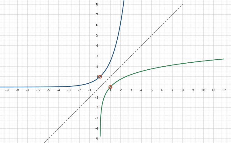
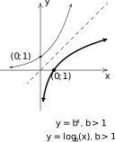
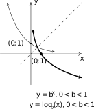
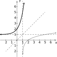
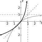
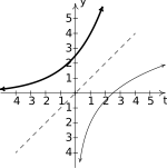
Since logs are defined as the inverses of exponential functions, we can use Theorems 5.13 and 7.1 to tell us about logarithmic functions. For example, we know that the domain of a log function is the range of an exponential function, namely $open parenthesis 0, ∞ close parenthesis$ , and that the range of a log function is the domain of an exponential function, namely $open parenthesis minus ∞, ∞ close parenthesis$ .

Moreover, since we know the basic shapes of $y = f (x) = b^{x}$ for the different cases of $b$ , we can obtain the graph of $y = f^{- 1} (x) = \log_{b} (x)$ by reflecting the graph of $f$ across the line $y = x$ . The $y$ -intercept $open parenthesis 0, 1 close parenthesis$ on the graph of $f$ corresponds to an $x$ -intercept of $open parenthesis 1, 0 close parenthesis$ on the graph of $f^{- 1}$ . The horizontal asymptotes $y equals 0$ on the graphs of the exponential functions become vertical asymptotes $x equals 0$ on the log graphs.

Coordinate-plane figure. — **Figure 7.28**

Procedurally, logarithmic functions `undo' the exponential functions. Consider the function $f (x) = 2^{x}$ . When we evaluate $f (3) = 2^{3} = 8$ , the input $3$ becomes the exponent on the base $2$ to produce the real number $8$ . The function $f^{- 1} (x) = \log_{2} (x)$ then takes the number $8$ as its input and returns the exponent $3$ as its output. In symbols, $log sub 2 ⁡ open parenthesis 8 close parenthesis equals 3$ .

More generally, $log sub 2 ⁡ open parenthesis x close parenthesis$ is the exponent you put on $2$ to get $x$ . Thus, $log sub 2 ⁡ open parenthesis 16 close parenthesis equals 4$ , because $2^{4} = 16$ . The following theorem summarizes the basic properties of logarithmic functions, all of which come from the fact that they are inverses of exponential functions.

Theorem

Properties of Logarithmic Functions: Suppose $f (x) = \log_{b} (x)$ .

The domain of $f$ is $open parenthesis 0, ∞ close parenthesis$ and the range of $f$ is $open parenthesis minus ∞, ∞ close parenthesis$ .
$open parenthesis 1, 0 close parenthesis$ is on the graph of $f$ and $x equals 0$ is a vertical asymptote of the graph of $f$ .
$f$ is one-to-one, continuous and smooth
$b^{a} = c$ if and only if $\log_{b} (c) = a$ . That is, $\log_{b} (c)$ is the exponent you put on $b$ to obtain $c$ .
$\log_{b} (b^{x}) = x$ for all real numbers $x$ and $b^{\log_{b} (x)} = x$ for all $x greater than 0$

If $b greater than 1$ :
- $f$ is always increasing
- $lim_{x \to 0^{+}} f (x) = - \infty$
- $lim x → ∞ f ⁢ open parenthesis x close parenthesis equals ∞$
- The graph of $f$ resembles:
  Figure 7.30

If $0 less than b less than 1$ :
- $f$ is always decreasing
- $lim_{x \to 0^{+}} f (x) = \infty$
- $lim_{x \to \infty} f (x) = - \infty$
- The graph of $f$ resembles:
  Figure 7.31

As we have mentioned, Theorem 7.3 is a consequence of Theorems 5.13 and 7.1. However, it is worth the reader's time to understand Theorem 7.3 from an exponent perspective.

As an example, we know that the domain of $g ⁢ open parenthesis x close parenthesis equals log sub 2 ⁡ open parenthesis x close parenthesis$ is $open parenthesis 0, ∞ close parenthesis$ . Why? Because the range of $f (x) = 2^{x}$ is $open parenthesis 0, ∞ close parenthesis$ . In a way, this says everything, but at the same time, it doesn't.

To really understand why the domain of $g ⁢ open parenthesis x close parenthesis equals log sub 2 ⁡ open parenthesis x close parenthesis$ is $open parenthesis 0, ∞ close parenthesis$ , consider trying to compute $log sub 2 ⁡ open parenthesis minus 1 close parenthesis$ . We are searching for the exponent we put on $2$ to give us $minus 1$ . In other words, we are looking for $x$ that satisfies $2^{x} = - 1$ . There is no such real number, since all powers of $2$ are positive.

While what we have said is exactly the same thing as saying `the domain of $g ⁢ open parenthesis x close parenthesis equals log sub 2 ⁡ open parenthesis x close parenthesis$ is $open parenthesis 0, ∞ close parenthesis$ because the range of $f (x) = 2^{x}$ is $open parenthesis 0, ∞ close parenthesis$ ', we feel it is in a student's best interest to understand the statements in Theorem 7.3 at this level instead of just merely memorizing the facts.

Our first example gives us practice computing logarithms as well as constructing basic graphs.

Example 1

Simplify the following.
1. $log sub 3 ⁡ open parenthesis 81 close parenthesis$
2. $\log_{2} (\frac{1}{8})$
3. $log sub the square root of 5 ⁡ open parenthesis 25 close parenthesis$
4. $\ln (\sqrt[3]{e^{2}})$
5. $log ⁡ open parenthesis 0.001 close parenthesis$
6. $2 to the power log sub 2 ⁡ open parenthesis 8 close parenthesis$
7. $117^{- \log_{117} (6)}$
Graph the following functions by starting with a basic logarithmic function and using transformations, Theorem 5.11. Track at least three points and the vertical asymptote through the transformations.
1. $F (x) = \log_{\frac{1}{3}} (\frac{x}{2}) + 1$
2. $G (t) = - \ln (2 - t)$
Find a formula for the graph of the function below. Assume the base of the logarithm is $2$ .
Figure 7.32 $y = F (x)$

1. The number $log sub 3 ⁡ open parenthesis 81 close parenthesis$ is the exponent we put on $3$ to get $81$ . As such, we want to write $81$ as a power of $3$ . We find $81 = 3^{4}$ , so that $log sub 3 ⁡ open parenthesis 81 close parenthesis equals 4$ .
2. To find $\log_{2} (\frac{1}{8})$ , we need rewrite $\frac{1}{8}$ as a power of $2$ . We find $\frac{1}{8} = \frac{1}{2^{3}} = 2^{- 3}$ , so $\log_{2} (\frac{1}{8}) = - 3$ .
3. To determine $log sub the square root of 5 ⁡ open parenthesis 25 close parenthesis$ , we need to express $25$ as a power of $the square root of 5$ . We know $25 equals 5 squared$ , and $5 = {(\sqrt{5})}^{2}$ , so we have $25 = {({(\sqrt{5})}^{2})}^{2} = {(\sqrt{5})}^{4}$ . We get $\log_{\sqrt{5}} (25) = 4$ .
4. First, recall that the notation $\ln (\sqrt[3]{e^{2}})$ means $\log_{e} (\sqrt[3]{e^{2}})$ , so we are looking for the exponent to put on $e$ to obtain $\sqrt[3]{e^{2}}$ . Rewriting $\sqrt[3]{e^{2}} = e^{2 / 3}$ , we find $\ln (\sqrt[3]{e^{2}}) = \ln (e^{2 / 3}) = \frac{2}{3}$ .
5. Rewriting $log ⁡ open parenthesis 0.001 close parenthesis$ as $log sub 10 ⁡ open parenthesis 0.001 close parenthesis$ , we see that we need to write $0.001$ as a power of $10$ . We have $0.001 = \frac{1}{1000} = \frac{1}{10^{3}} = 10^{- 3}$ . Hence, $\log (0.001) = \log (10^{- 3}) = - 3$ .
6. We can use Theorem 7.3 directly to simplify $2^{\log_{2} (8)} = 8$ .
  We can also understand this problem by first finding $log sub 2 ⁡ open parenthesis 8 close parenthesis$ . By definition, $log sub 2 ⁡ open parenthesis 8 close parenthesis$ is the exponent we put on $2$ to get $8$ . Since $8 equals 2 cubed$ , we have $log sub 2 ⁡ open parenthesis 8 close parenthesis equals 3$ .
  We now substitute to find $2^{\log_{2} (8)} = 2^{3} = 8$ .
7. From Theorem 7.3, we know $117^{\log_{117} (6)} = 6$ ,¹ but we cannot directly apply this formula to the expression $117^{- \log_{117} (6)}$ without first using a property of exponents. (Can you see why?)
  Rather, we find: $117^{- \log_{117} (6)} = \frac{1}{117^{\log_{117} (6)}} = \frac{1}{6}$ .
1. To graph $F (x) = \log_{\frac{1}{3}} (\frac{x}{2}) + 1$ we start with the graph of $f (x) = \log_{\frac{1}{3}} (x)$ . and use Theorem 5.11.
  First we choose some `control points' on the graph of $f (x) = \log_{\frac{1}{3}} (x)$ . Since we are instructed to track three points (and the vertical asymptote, $x equals 0$ ) through the transformations, we choose the points corresponding to powers of $\frac{1}{3}$ : $(\frac{1}{3}, 1)$ , $open parenthesis 1, 0 close parenthesis$ , and $open parenthesis 3, minus 1 close parenthesis$ , respectively.
  Next, we note $F (x) = \log_{\frac{1}{3}} (\frac{x}{2}) + 1 = f (\frac{x}{2}) + 1$ . Per Theorem 5.11, we first multiply the $x$ -coordinates of the points on the graph of $y = f (x)$ by $2$ , horizontally expanding the graph by a factor of $2$ . Next, we add $1$ to the $y$ -coordinates of each point on this new graph, vertically shifting the graph up $1$ .
  Looking at each point, we get $(\frac{1}{3}, 1) \to (\frac{2}{3}, 1) \to (\frac{2}{3}, 2)$ , $open parenthesis 1, 0 close parenthesis → open parenthesis 2, 0 close parenthesis → open parenthesis 2, 1 close parenthesis$ , and $(3, - 1) \to (6, - 1) \to (6, 0)$ . The horizontal asymptote, $x equals 0$ remains unchanged under the horizontal stretch and the vertical shift.
  Below we graph $y = f (x) = \log_{\frac{1}{3}} (x)$ on the left and $y = F (x) = \log_{\frac{1}{3}} (\frac{x}{2}) + 1$ on the right.
  Figure 7.33 $y = f (x) = \log_{\frac{1}{3}} (x)$
  
  Figure 7.34 $y = F (x) = \log_{\frac{1}{3}} (\frac{x}{2}) + 1$
  As always we can check our answer by verifying each of the points $(\frac{2}{3}, 2)$ , $open parenthesis 2, 1 close parenthesis$ ,, and $open parenthesis 6, 0 close parenthesis$ , is on the graph of $F (x) = \log_{\frac{1}{3}} (\frac{x}{2}) + 1$ by checking $F (\frac{2}{3}) = 2$ , $F ⁢ open parenthesis 2 close parenthesis equals 1$ , and $F ⁢ open parenthesis 6 close parenthesis equals 0$ . We can check the end behavior as well, that is, $lim_{x \to 0^{+}} F (x) = \infty$ and as $lim x → ∞ F ⁢ open parenthesis x close parenthesis → minus ∞$ . We leave these calculations to the reader.
2. Since the base of $G (t) = - \ln (2 - t)$ is $e$ , we start with the graph of $g (t) = \ln (t)$ . As usual, since $e$ is an irrational number, we use the approximation $e approximately equals 2.718$ when plotting points, but label points using exact coordinates in terms of $e$ .
  We choose points corresponding to powers of $e$ on the graph of $g (t) = \ln (t)$ : $(e^{- 1}, - 1) \approx (0.368, - 1)$ , $open parenthesis 1, 0 close parenthesis$ , and $open parenthesis e, 1 close parenthesis approximately equals open parenthesis 2.718, 1 close parenthesis$ , respectively.
  Since $G (t) = - \ln (2 - t) = - \ln (- t + 2) = - g (- t + 2)$ , Theorem 5.11 instructs us to first subtract $2$ from each of the $t$ -coordinates of the points on the graph of $g (t) = \ln (t)$ , shifting the graph to the left two units.
  Next, we multiply (divide) the $t$ -coordinates of points on this new graph by $minus 1$ which reflects the graph across the $y$ -axis. Lastly, we multiply each of the $y$ -coordinates of this second graph by $minus 1$ , reflecting it across the $t$ -axis.
  Tracking points, we have $(e^{- 1}, - 1) \to (e^{- 1} - 2, - 1) \to (- e^{- 1} + 2, - 1) \to (- e^{- 1} + 2, 1) \approx (1.632, 1)$ , $open parenthesis 1, 0 close parenthesis → open parenthesis minus 1, 0 close parenthesis → open parenthesis 1, 0 close parenthesis → open parenthesis 1, 0 close parenthesis$ , and $(e, 1) \to (e - 2, 1) \to (- e + 2, 1) \to (- e + 2, - 1) \approx (- 0.718, - 1)$ . The vertical asymptote is affected by the horizontal shift and the reflection about the $y$ -axis only: $t = 0 \to t = - 2 \to t = 2$ .
  We graph $g (t) = \ln (t)$ below on the left and the transformed function $G (t) = - \ln (- t + 2)$ below on the right. As usual, we can check our answer by verifying the indicated points do, in fact, lie on the graph of $y = G (t)$ along with checking the behavior as $t → minus ∞$ and $t \to 2^{-}$ .
  Figure 7.35 $y = g (t) = \ln (t)$
  
  Figure 7.36 $y = G (t) = - \ln (- t + 2)$
Since we are told to assume the base of the exponential function is $2$ , we assume the function $F (x)$ is the result of the transforming the graph of $f ⁢ open parenthesis x close parenthesis equals log sub 2 ⁡ open parenthesis x close parenthesis$ using Theorem 5.11. This means we are tasked with finding values for $a$ , $b$ , $h$ , and $k$ so that $F (x) = a f (b x - h) + k = a \log_{2} (b x - h) + k$ .
Since the vertical asymptote to the graph of $y = f (x) = \log_{2} (x)$ is $x equals 0$ and the vertical asymptote to the graph $y = F (x)$ is $x equals 4$ , we know we have a vertical shift of $4$ units. Moreover, since the curve approaches the vertical asymptote from the left, we also know we have a reflection about the $y$ -axis, so $b less than 0$ . Since the recipe in Theorem 5.11 instructs us to perform the vertical shift before the reflection across the $y$ -axis, we take $h = - 4$ and assume for simplicity $b = - 1$ so $F (x) = a \log_{2} (- x + 4) + k$ .
To determine $a$ and $k$ , we make use of the two points on the graph. Since $open parenthesis minus 4, 0 close parenthesis$ is on the graph of $F$ , $F (- 4) = a \log_{2} (- (- 4) + 4) + k = 0$ . This reduces to $a \log_{2} (8) + k = 0$ or $3 a + k = 0$ . Next, we use the point $open parenthesis 0, minus 1 close parenthesis$ to get $F (0) = a \log_{2} (- (0) + 4) + k = - 1$ . This reduces to $a \log_{2} (4) + k = - 1$ or $2 a + k = - 1$ . From $3 a + k = 0$ , we get $k = - 3 a$ which when substituted into $2 a + k = - 1$ gives $2 a + (- 3 a) = - 1$ or $a equals 1$ . Hence, $k = - 3 a = - 3 (1) = - 3$ .
Putting all of this work together we find $F (x) = \log_{2} (- x + 4) - 3$ . As always, we can check our answer by verifying $F (- 4) = 0$ , $F (0) = - 1$ , $lim_{x \to - \infty} F (x) = \infty$ , and $lim_{x \to 4^{-}} F (x) = - \infty$ . We leave these details to the reader.²

Up until this point, restrictions on the domains of functions came from avoiding division by zero and keeping negative numbers from beneath even indexed radicals. With the introduction of logs, we now have another restriction. Since the domain of $f (x) = \log_{b} (x)$ is $open parenthesis 0, ∞ close parenthesis$ , the argument of the log³ must be strictly positive.

Example 2

Find the domain each function analytically and check your answer using a graphing utility.

$f (x) = 2 \log (3 - x) - 1$
$g (x) = \ln (\frac{x}{x - 1})$

We set $3 minus x greater than 0$ to obtain $x less than 3$ , or $open parenthesis minus ∞, 3 close parenthesis$ as confirmed by our graphing utility below.
Figure 7.37
Note that in this case, we can graph $f$ using transformations, which we do so here for extra practice.
Taking a cue from Theorem 5.11, we rewrite $f (x) = 2 \log_{10} (- x + 3) - 1$ and view this function as a transformed version of $h ⁢ open parenthesis x close parenthesis equals log sub 10 ⁡ open parenthesis x close parenthesis$ .
To graph $y = \log (x) = \log_{10} (x)$ , We select three points to track corresponding to powers of $10$ : $open parenthesis 0.1, minus 1 close parenthesis$ , $open parenthesis 1, 0 close parenthesis$ and $open parenthesis 10, 1 close parenthesis$ , along with the vertical asymptote $x equals 0$ .
Since $f (x) = 2 h (- x + 3) - 1$ , Theorem 5.11 tells us that to obtain the destinations of these points, we first subtract $3$ from the $x$ -coordinates (shifting the graph left $3$ units), then divide (multiply) by the $x$ -coordinates by $minus 1$ (causing a reflection across the $y$ -axis).
Next, we multiply the $y$ -coordinates by $2$ which results in a vertical stretch by a factor of $2$ , then we finish by subtracting $1$ from the $y$ -coordinates which shifts the graph down $1$ unit.
Tracking points, we find: $(0.1, - 1) \to (- 2.9, - 1) \to (2.9, - 1) \to (2.9, - 2) \to (2.9, - 3)$ , $(1, 0) \to (- 2, 0) \to (2, 0) \to (2, 0) \to (2, - 1)$ , and $(10, 1) \to (7, 1) \to (- 7, 1) \to (- 7, 2) \to (- 7, 1)$ . The vertical shift and reflection about the $y$ -axis affects the vertical asymptote: $x = 0 \to x = - 3 \to x = 3$ .
Plotting these three points along with the vertical asymptote produces the graph of $f$ as seen above.
To find the domain of $g$ , we need to solve the inequality $\frac{x}{x - 1} > 0$ using a sign diagram.⁴
If we define $r (x) = \frac{x}{x - 1}$ , we find $r$ is undefined at $x equals 1$ and $r ⁢ open parenthesis x close parenthesis equals 0$ when $x equals 0$ . Choosing some test values, we generate the sign diagram below on the left.
We find $\frac{x}{x - 1} > 0$ on $open parenthesis minus ∞, 0 close parenthesis union open parenthesis 1, ∞ close parenthesis$ which is the domain of $g$ . The graph below confirms this.
Figure 7.38
Figure 7.39
We can tell from the graph of $g$ that it is not the result of Section 5.4 transformations being applied to the graph $y = \ln (x)$ , (do you see why?) so barring a more detailed analysis using Calculus, producing a graph using a graphing utility is the best we can do.
One thing worthy of note, however, is the end behavior of $g$ . The graph suggests that $lim_{x \to - \infty} g (x) = 0$ and $lim x → ∞ g ⁢ open parenthesis x close parenthesis equals 0$ . We can verify this analytically. Using results from Chapter 3 and continuity, we know that $lim_{x \to - \infty} \frac{x}{x + 1} = 1$ and $lim_{x \to \infty} \frac{x}{x + 1} = 1$ . Hence, it stands to reason that
$lim_{x \to - \infty} g (x) = lim_{x \to - \infty} \ln (\frac{x}{x - 1}) = l n (1) = 0$
and, likewise, $lim_{x \to - \infty} g (x) = l n (1) = 0$ .

While logarithms have some interesting applications of their own which you'll explore in the exercises, their primary use to us will be to undo exponential functions. (This is, after all, how they were defined.) Our last example reviews not only the major topics of this section, but reviews the salient points from Section 5.6.

Example 3

Let $f (x) = 2^{x - 1} - 3$ .

Graph $f$ using transformations and state the domain and range of $f$ .
Explain why $f$ is invertible and find a formula for $f^{- 1} (x)$ .
Graph $f^{- 1}$ using transformations and state the domain and range of $f^{- 1}$ .
Verify $(f^{- 1} \circ f) (x) = x$ for all $x$ in the domain of $f$ and $(f \circ f^{- 1}) (x) = x$ for all $x$ in the domain of $f^{- 1}$ .
Graph $f$ and $f^{- 1}$ on the same set of axes and check for symmetry about the line $y = x$ .
Use $f$ or $f^{- 1}$ to solve the following equations. Check your answers algebraically.
1. $2^{x - 1} - 3 = 4$
2. $\log_{2} (t + 3) + 1 = 0$

To graph $f (x) = 2^{x - 1} - 3$ using Theorem 5.11, we first identify $g (x) = 2^{x}$ and note $f (x) = g (x - 1) - 3$ . Choosing the `control points' of $(- 1, \frac{1}{2})$ , $open parenthesis 0, 1 close parenthesis$ and $open parenthesis 1, 2 close parenthesis$ on the graph of $g$ along with the horizontal asymptote $y equals 0$ , we implement the algorithm set forth in Theorem 5.11.
First, we first add $1$ to the $x$ -coordinates of the points on the graph of $g$ which shifts the the graph of $g$ to the right one unit. Next, we subtract $3$ from each of the $y$ -coordinates on this new graph, shifting the graph down $3$ units to get the graph of $f$ .
Looking point-by-point, we have $(- 1, \frac{1}{2}) \to (0, \frac{1}{2}) \to (0, - \frac{5}{2})$ , $open parenthesis 0, 1 close parenthesis → open parenthesis 1, 1 close parenthesis → open parenthesis 1, minus 2 close parenthesis$ , and, finally, $open parenthesis 1, 2 close parenthesis → open parenthesis 2, 2 close parenthesis → open parenthesis 2, minus 1 close parenthesis$ . The horizontal asymptote is affected only by the vertical shift, $y = 0 \to y = - 3$ .
From the graph of $f$ , we get the domain is $open parenthesis minus ∞, ∞ close parenthesis$ and the range is $open parenthesis minus 3, ∞ close parenthesis$ .
Figure 7.40 $y = h (x) = 2^{x}$
$\overset{}{\to}$
Figure 7.41 $y = f (x) = 2^{x - 1} - 3$
The graph of $f$ passes the Horizontal Line Test so $f$ is one-to-one, hence invertible.
To find a formula for $f^{- 1} (x)$ , we normally set $y = f (x)$ , interchange the $x$ and $y$ , then proceed to solve for $y$ . Doing so in this situation leads us to the equation $x = 2^{y - 1} - 3$ . We have yet to discuss how to solve this kind of equation, so we will attempt to find the formula for $f^{- 1}$ procedurally.
Thinking of $f$ as a process, the formula $f (x) = 2^{x - 1} - 3$ takes an input $x$ and applies the steps: first subtract $1$ . Second put the result of the first step as the exponent on $2$ . Last, subtract $3$ from the result of the second step.
Clearly, to undo subtracting $1$ , we will add $1$ , and similarly we undo subtracting $3$ by adding $3$ . How do we undo the second step? The answer is we use the logarithm.
By definition, $log sub 2 ⁡ open parenthesis x close parenthesis$ undoes exponentiation by $2$ . Hence, $f^{- 1}$ should: first, add $3$ . Second, take the logarithm base $2$ of the result of the first step. Lastly, add $1$ to the result of the second ste. In symbols, $f^{- 1} (x) = \log_{2} (x + 3) + 1$ .
To graph $f^{- 1} (x) = \log_{2} (x + 3) + 1$ using Theorem 5.11, we start with $j ⁢ open parenthesis x close parenthesis equals log sub 2 ⁡ open parenthesis x close parenthesis$ and track the points $(\frac{1}{2}, - 1)$ , $open parenthesis 1, 0 close parenthesis$ and $open parenthesis 2, 1 close parenthesis$ on the graph of $j$ along with the vertical asymptote $x equals 0$ through the transformations.
Since $f^{- 1} (x) = j (x + 3) + 1$ , we first subtract $3$ from each of the $x$ -coordinates of each of the points on the graph of $y = j (x)$ shifting the graph of $j$ to the left three units. We then add $1$ to each of the $y$ -coordinates of the points on this new graph, shifting the graph up one unit.
Tracking points, we get $(\frac{1}{2}, - 1) \to (- \frac{5}{2}, - 1) \to (- \frac{5}{2}, 0)$ , $(1, 0) \to (- 2, 1) \to (- 2, 2)$ , and $(2, 1) \to (- 1, 1) \to (- 1, 2)$ .
The vertical asymptote is only affected by the horizontal shift, so we have $x = 0 \to x = - 3$ .
From the graph below, we get the domain of $f^{- 1}$ is $open parenthesis minus 3, ∞ close parenthesis$ , which matches the range of $f$ , and the range of $f^{- 1}$ is $open parenthesis minus ∞, ∞ close parenthesis$ , which matches the domain of $f$ , in accordance with Theorem 5.13.
Figure 7.42 $y = j (x) = \log_{2} (x)$
$\overset{}{\to}$
Figure 7.43 $y = f^{- 1} (x) = \log_{2} (x + 3) + 1$
We now verify that $f (x) = 2^{x - 1} - 3$ and $f^{- 1} (x) = \log_{2} (x + 3) + 1$ satisfy the composition requirement for inverses. When simplifying $(f^{- 1} \circ f) (x)$ we assume $x$ can be any real number while when simplifying $(f \circ f^{- 1}) (x)$ , we restrict our attention to $x greater than minus 3$ . (Do you see why?)
Note the use of the inverse properties of exponential and logarithmic functions from Theorem 7.3 when it comes to simplifying expressions of the form $log sub 2 ⁡ open parenthesis 2 to the power u close parenthesis$ and $2 to the power log sub 2 ⁡ open parenthesis u close parenthesis$ .
$\begin{matrix} (f^{- 1} \circ f) (x) & = & f^{- 1} (f (x)) \\ = & f^{- 1} (2^{x - 1} - 3) \\ = & \log_{2} ([2^{x - 1} - 3] + 3) + 1 \\ = & \log_{2} (2^{x - 1}) + 1 \\ = & (x - 1) + 1 \\ = & x ✓ \end{matrix}$
$\begin{matrix} (f \circ f^{- 1}) (x) & = & f (f^{- 1} (x)) \\ = & f (\log_{2} (x + 3) + 1) \\ = & 2^{(\log_{2} (x + 3) + 1) - 1} - 3 \\ = & 2^{\log_{2} (x + 3)} - 3 \\ = & (x + 3) - 3 \\ = & x ✓ \end{matrix}$
Last, but certainly not least, we graph $y = f (x)$ and $y = f^{- 1} (x)$ on the same set of axes and observe the symmetry about the line $y = x$ .
Figure 7.44

Viewing $2^{x - 1} - 3 = 4$ as $f ⁢ open parenthesis x close parenthesis equals 4$ , we apply $f^{- 1}$ to `undo' $f$ to get $f^{- 1} (f (x)) = f^{- 1} (4)$ , which reduces to $x = f^{- 1} (4)$ . Since we have shown (algebraically and graphically!) that $f^{- 1} (x) = \log_{2} (x + 3) + 1$ , we get $x = f^{- 1} (4) = \log_{2} (4 + 3) + 1 = \log_{2} (7) + 1$ .
Alternatively, we know from Theorem 5.13 that $f ⁢ open parenthesis x close parenthesis equals 4$ is equivalent to $x = f^{- 1} (4)$ directly.
Note that since, by definition, $2^{\log_{2} (7)} = 7$ , $2^{(\log_{2} (7) + 1) - 1} - 3 = 2^{\log_{2} (7)} - 3 = 7 - 3 = 4$ , as required.
Since we may think of the equation $\log_{2} (t + 3) + 1 = 0$ as $f^{- 1} (t) = 0$ , we can solve this equation by applying $f$ to both sides to get $f (f^{- 1} (t)) = f (0)$ or $t = 2^{0 - 1} - 3 = \frac{1}{2} - 3 = - \frac{5}{2}$ .
Since $\log_{2} (2^{- 1}) = - 1$ , we get $\log_{2} (- \frac{5}{2} + 3) + 1 = \log_{2} (\frac{1}{2}) + 1 = \log_{2} (2^{- 1}) - 1 + 1 = 0$ , as required.

Exercises

In Exercises -, use the property: $b^{a} = c$ if and only if $\log_{b} (c) = a$ from Theorem 7.3 to rewrite the given equation in the other form. That is, rewrite the exponential equations as logarithmic equations and rewrite the logarithmic equations as exponential equations.

$2 cubed equals 8$
$5^{- 3} = \frac{1}{125}$
$4^{5 / 2} = 32$
${(\frac{1}{3})}^{- 2} = 9$
${(\frac{4}{25})}^{- 1 / 2} = \frac{5}{2}$
$10^{- 3} = 0.001$
$e^{0} = 1$
$log sub 5 ⁡ open parenthesis 25 close parenthesis equals 2$
$\log_{25} (5) = \frac{1}{2}$
$\log_{3} (\frac{1}{81}) = - 4$
$\log_{\frac{4}{3}} (\frac{3}{4}) = - 1$
$log ⁡ open parenthesis 100 close parenthesis equals 2$
$\log (0.1) = - 1$
$ln ⁡ open parenthesis e close parenthesis equals 1$
$\ln (\frac{1}{\sqrt{e}}) = - \frac{1}{2}$

In Exercises -, evaluate the expression without using a calculator.

$log sub 3 ⁡ open parenthesis 27 close parenthesis$
$log sub 6 ⁡ open parenthesis 216 close parenthesis$
$log sub 2 ⁡ open parenthesis 32 close parenthesis$
$\log_{6} (\frac{1}{36})$
$log sub 8 ⁡ open parenthesis 4 close parenthesis$
$log sub 36 ⁡ open parenthesis 216 close parenthesis$
$\log_{\frac{1}{5}} (625)$
$\log_{\frac{1}{6}} (216)$
$log sub 36 ⁡ open parenthesis 36 close parenthesis$
$\log (\frac{1}{1000000})$
$log ⁡ open parenthesis 0.01 close parenthesis$
$\ln (e^{3})$
$log sub 4 ⁡ open parenthesis 8 close parenthesis$
$log sub 6 ⁡ open parenthesis 1 close parenthesis$
$log sub 13 ⁡ open parenthesis the square root of 13 close parenthesis$
$log sub 36 ⁡ open parenthesis the 4th root of 36 close parenthesis$
$7 to the power log sub 7 ⁡ open parenthesis 3 close parenthesis$
$36 to the power log sub 36 ⁡ open parenthesis 216 close parenthesis$
$log sub 36 ⁡ open parenthesis 36 to the power 216 close parenthesis$
$ln ⁡ open parenthesis e to the power 5 close parenthesis$
$\log (\sqrt[9]{10^{11}})$
$\log (\sqrt[3]{10^{5}})$
$\ln (\frac{1}{\sqrt{e}})$
$log sub 5 ⁡ open parenthesis 3 to the power log sub 3 ⁡ open parenthesis 5 close parenthesis close parenthesis$
$log ⁡ open parenthesis e to the power ln ⁡ open parenthesis 100 close parenthesis close parenthesis$
$\log_{2} (3^{- \log_{3} (2)})$
$ln ⁡ open parenthesis 42 to the power 6 ⁢ log ⁡ open parenthesis 1 close parenthesis close parenthesis$

In Exercises -, find the domain of the function.

$f (x) = \ln (x^{2} + 1)$
$f (x) = \log_{7} (4 x + 8)$
$g (t) = \ln (4 t - 20)$
$g (t) = \log (t^{2} + 9 t + 18)$
$f (x) = \log (\frac{x + 2}{x^{2} - 1})$
$f (x) = \log (\frac{x^{2} + 9 x + 18}{4 x - 20})$
$g (t) = \ln (7 - t) + \ln (t - 4)$
$g (t) = \ln (4 t - 20) + \ln (t^{2} + 9 t + 18)$
$f (x) = \log (x^{2} + x + 1)$
$f (x) = \sqrt[4]{\log_{4} (x)}$
$g (t) = \log_{9} (| t + 3 | - 4)$
$g (t) = \ln (\sqrt{t - 4} - 3)$
$f (x) = \frac{1}{3 - \log_{5} (x)}$
$f (x) = \frac{\sqrt{- 1 - x}}{\log_{\frac{1}{2}} (x)}$
$f (x) = \ln (- 2 x^{3} - x^{2} + 13 x - 6)$

In Exercises -, sketch the graph of $g$ by starting with the graph of $f$ and using transformations. Track at least three points of your choice and the vertical asymptote through the transformations. State the domain and range of $g$ .

$f ⁢ open parenthesis x close parenthesis equals log sub 2 ⁡ open parenthesis x close parenthesis$ , $g (x) = \log_{2} (x + 1)$
$f (x) = \log_{\frac{1}{3}} (x)$ , $g (x) = \log_{\frac{1}{3}} (x) + 1$
$f ⁢ open parenthesis x close parenthesis equals log sub 3 ⁡ open parenthesis x close parenthesis$ , $g (x) = - \log_{3} (x - 2)$
$f (x) = \log (x)$ , $g (x) = 2 \log (x + 20) - 1$
$f ⁢ open parenthesis t close parenthesis equals log sub 0.5 ⁡ open parenthesis t close parenthesis$ , $g (t) = 10 \log_{0.5} (\frac{t}{100})$
$f ⁢ open parenthesis t close parenthesis equals log sub 1.25 ⁡ open parenthesis t close parenthesis$ , $g (t) = \log_{1.25} (- t + 1) + 2$
$f (t) = \ln (t)$ , $g (t) = - \ln (8 - t)$
$f (t) = \ln (t)$ , $g (t) = - 10 \ln (\frac{t}{10})$
Verify that each function in Exercises - is the inverse of the corresponding function in Exercises - in Section 7.1. (Match up # and #, and so on.)

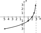
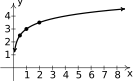
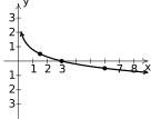
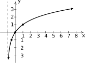
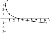
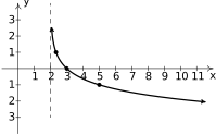
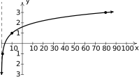
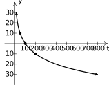
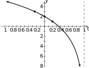
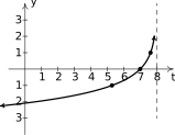
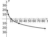
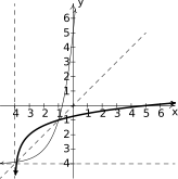
In Exercises, -, the graph of a logarithmic function is given. Find a formula for the function in the form $F (x) = a \cdot \log_{2} (b x - h) + k$ .

Points: $(- \frac{5}{2}, - 2)$ , $(- 2, - 1)$ , $open parenthesis minus 1, 0 close parenthesis$ , Asymptote: $x = - 3$ .
Figure 7.45
Points: $open parenthesis 1, minus 1 close parenthesis$ , $open parenthesis 2, 0 close parenthesis$ , $(\frac{5}{2}, 1)$ Asymptote: $x equals 3$ .
Figure 7.46
Points: $(\frac{1}{2}, \frac{5}{2})$ , $open parenthesis 1, 3 close parenthesis$ , $(2, \frac{7}{2})$ , Asymptote: $x equals 0$ .
Figure 7.47
Points: $(6, - \frac{1}{2})$ , $open parenthesis 3, 0 close parenthesis$ , $(\frac{3}{2}, \frac{1}{2})$ , Asymptote: $x equals 0$ .
Figure 7.48
Find a formula for each graph in Exercises - of the form $G (x) = a \cdot \log_{4} (b x - h) + k$ .

In Exercises -, find the inverse of the function from the `procedural perspective' discussed in Example 7.2.3 and graph the function and its inverse on the same set of axes.

$f (x) = 3^{x + 2} - 4$
$f (x) = \log_{4} (x - 1)$
$g (t) = - 2^{- t} + 1$
$g (t) = 5 \log (t) - 2$

In Exercises -, write the given function as a nontrivial decomposition of functions as directed.

For $f (x) = \log_{2} (x + 3) + 4$ , find functions $g$ and $h$ so that $f = g + h$ .
For $f (x) = \log (2 x) - e^{- x}$ , find functions $g$ and $h$ so that $f = g - h$ .
For $f ⁢ open parenthesis t close parenthesis equals 3 ⁢ t ⁢ log ⁡ open parenthesis t close parenthesis$ , find functions $g$ and $h$ so that $f = g h$ .
For $r (x) = \frac{\ln (x)}{x}$ , find functions $f$ and $g$ so $r = \frac{f}{g}$ .
For $k (t) = \ln (t^{2} + 1)$ , find functions $f$ and $g$ so that $k equals g ∘ f$ .
For $p (z) = {(\ln (z))}^{2}$ , find functions $f$ and $g$ so $p equals g ∘ f$ .

(Logarithmic Scales) In Exercises -, we introduce three widely used measurement scales which involve common logarithms: the Richter scale, the decibel scale and the pH scale. The computations involved in all three scales are nearly identical so pay attention to the subtle differences.

Earthquakes are complicated events and it is not our intent to provide a complete discussion of the science involved in them. Instead, we refer the interested reader to a solid course in Geology⁵ or the U.S. Geological Survey's Earthquake Hazards Program found here and present only a simplified version of the Richter scale . The Richter scale measures the magnitude of an earthquake by comparing the amplitude of the seismic waves of the given earthquake to those of a “magnitude 0 event”, which was chosen to be a seismograph reading of $0.001$ millimeters recorded on a seismometer 100 kilometers from the earthquake's epicenter. Specifically, the magnitude of an earthquake is given by
$M (x) = \log (\frac{x}{0.001})$
where $x$ is the seismograph reading in millimeters of the earthquake recorded 100 kilometers from the epicenter.
1. Show that $M ⁢ open parenthesis 0.001 close parenthesis equals 0$ .
2. Compute $M ⁢ open parenthesis 80, 000 close parenthesis$ .
3. Show that an earthquake which registered 6.7 on the Richter scale had a seismograph reading ten times larger than one which measured 5.7.
4. Find two news stories about recent earthquakes which give their magnitudes on the Richter scale. How many times larger was the seismograph reading of the earthquake with larger magnitude?
While the decibel scale can be used in many disciplines,⁶ we shall restrict our attention to its use in acoustics, specifically its use in measuring the intensity level of sound. The Sound Intensity Level $L$ (measured in decibels) of a sound intensity $I$ (measured in watts per square meter) is given by
$L (I) = 10 \log (\frac{I}{10^{- 12}}) .$
Like the Richter scale, this scale compares $I$ to baseline: $10^{- 12} \frac{W}{m^{2}}$ is the threshold of human hearing.
1. Compute $L (10^{- 6})$ .
2. Damage to your hearing can start with short term exposure to sound levels around 115 decibels. What intensity $I$ is needed to produce this level?
3. Compute $L ⁢ open parenthesis 1 close parenthesis$ . How does this compare with the threshold of pain which is around 140 decibels?
The pH of a solution is a measure of its acidity or alkalinity. Specifically, $pH = - \log [H^{+}]$ where $[H^{+}]$ is the hydrogen ion concentration in moles per liter. A solution with a pH less than 7 is an acid, one with a pH greater than 7 is a base (alkaline) and a pH of 7 is regarded as neutral.
1. The hydrogen ion concentration of pure water is $[H^{+}] = 10^{- 7}$ . Find its pH.
2. Find the pH of a solution with $[H^{+}] = 6.3 \times 10^{- 13}$ .
3. The pH of gastric acid (the acid in your stomach) is about $0.7$ . What is the corresponding hydrogen ion concentration?
Use the definition of logarithm to explain why $log sub b ⁡ 1 equals 0$ and $log sub b ⁡ b equals 1$ for every $b greater than 0, b not equal to 1$ .

Answers

$log sub 2 ⁡ open parenthesis 8 close parenthesis equals 3$
$\log_{5} (\frac{1}{125}) = - 3$
$\log_{4} (32) = \frac{5}{2}$
$\log_{\frac{1}{3}} (9) = - 2$
$\log_{\frac{4}{25}} (\frac{5}{2}) = - \frac{1}{2}$
$\log (0.001) = - 3$
$ln ⁡ open parenthesis 1 close parenthesis equals 0$
$5 squared equals 25$
${(25)}^{\frac{1}{2}} = 5$
$3^{- 4} = \frac{1}{81}$
${(\frac{4}{3})}^{- 1} = \frac{3}{4}$
$10 squared equals 100$
$10^{- 1} = 0.1$
$e^{1} = e$
$e^{- \frac{1}{2}} = \frac{1}{\sqrt{e}}$
$log sub 3 ⁡ open parenthesis 27 close parenthesis equals 3$
$log sub 6 ⁡ open parenthesis 216 close parenthesis equals 3$
$log sub 2 ⁡ open parenthesis 32 close parenthesis equals 5$
$\log_{6} (\frac{1}{36}) = - 2$
$\log_{8} (4) = \frac{2}{3}$
$\log_{36} (216) = \frac{3}{2}$
$\log_{\frac{1}{5}} (625) = - 4$
$\log_{\frac{1}{6}} (216) = - 3$
$log sub 36 ⁡ open parenthesis 36 close parenthesis equals 1$
$\log \frac{1}{1000000} = - 6$
$\log (0.01) = - 2$
$ln ⁡ open parenthesis e cubed close parenthesis equals 3$
$\log_{4} (8) = \frac{3}{2}$
$log sub 6 ⁡ open parenthesis 1 close parenthesis equals 0$
$\log_{13} (\sqrt{13}) = \frac{1}{2}$
$\log_{36} (\sqrt[4]{36}) = \frac{1}{4}$
$7^{\log_{7} (3)} = 3$
$36^{\log_{36} (216)} = 216$
$\log_{36} (36^{216}) = 216$
$\ln (e^{5}) = 5$
$\log (\sqrt[9]{10^{11}}) = \frac{11}{9}$
$\log (\sqrt[3]{10^{5}}) = \frac{5}{3}$
$\ln (\frac{1}{\sqrt{e}}) = - \frac{1}{2}$
$\log_{5} (3^{\log_{3} 5}) = 1$
$\log (e^{\ln (100)}) = 2$
$\log_{2} (3^{- \log_{3} (2)}) = - 1$
$\ln (42^{6 \log (1)}) = 0$
$open parenthesis minus ∞, ∞ close parenthesis$
$open parenthesis minus 2, ∞ close parenthesis$
$open parenthesis 5, ∞ close parenthesis$
$(- \infty, - 6) \cup (- 3, \infty)$
$(- 2, - 1) \cup (1, \infty)$
$(- 6, - 3) \cup (5, \infty)$
$open parenthesis 4, 7 close parenthesis$
$open parenthesis 5, ∞ close parenthesis$
$open parenthesis minus ∞, ∞ close parenthesis$
$open bracket 1, ∞ close parenthesis$
$(- \infty, - 7) \cup (1, \infty)$
$open parenthesis 13, ∞ close parenthesis$
$open parenthesis 0, 125 close parenthesis union open parenthesis 125, ∞ close parenthesis$
No domain
$(- \infty, - 3) \cup (\frac{1}{2}, 2)$
Domain of $g$ : $open parenthesis minus 1, ∞ close parenthesis$ Range of $g$ : $open parenthesis minus ∞, ∞ close parenthesis$ Points: $(- \frac{1}{2}, - 1)$ , $open parenthesis 0, 0 close parenthesis$ , $open parenthesis 1, 1 close parenthesis$ Asymptote: $x = - 1$
Figure 7.49 $y = g (x) = \log_{2} (x + 1)$
Domain of $g$ : $open parenthesis 0, ∞ close parenthesis$ Range of $g$ : $open parenthesis minus ∞, ∞ close parenthesis$ Points: $(\frac{1}{3}, 2)$ , $open parenthesis 1, 1 close parenthesis$ , $open parenthesis 3, 0 close parenthesis$ Asymptote: $x equals 0$
Figure 7.50 $y = g (x) = \log_{\frac{1}{3}} (x) + 1$
Domain of $g$ : $open parenthesis 2, ∞ close parenthesis$ Range of $g$ : $open parenthesis minus ∞, ∞ close parenthesis$ Points: $(\frac{7}{3}, 1)$ , $open parenthesis 3, 0 close parenthesis$ , $open parenthesis 5, minus 1 close parenthesis$ Asymptote: $x equals 2$
Figure 7.51 $y = g (x) = - \log_{3} (x - 2)$
Domain of $g$ : $open parenthesis minus 20, ∞ close parenthesis$ Range of $g$ : $open parenthesis minus ∞, ∞ close parenthesis$ Points: $(- 19, - 1)$ , $open parenthesis minus 10, 1 close parenthesis$ , $open parenthesis 80, 3 close parenthesis$ Asymptote: $x = - 20$
Figure 7.52 $y = g (x) = 2 \log (x + 20) - 1$
Domain of $g$ : $open parenthesis 0, ∞ close parenthesis$ Range of $g$ : $open parenthesis minus ∞, ∞ close parenthesis$ Points: $open parenthesis 50, 10 close parenthesis$ , $open parenthesis 100, 0 close parenthesis$ , $open parenthesis 200, minus 10 close parenthesis$ Asymptote: $t equals 0$
Figure 7.53 $y = g (t) = 10 \log_{0.5} (\frac{t}{100})$
Domain of $g$ : $open parenthesis minus ∞, 1 close parenthesis$ Range of $g$ : $open parenthesis minus ∞, ∞ close parenthesis$ Points: $open parenthesis minus 0.25, 3 close parenthesis$ , $open parenthesis 0, 2 close parenthesis$ , $open parenthesis 0.2, 1 close parenthesis$ Asymptote: $t equals 1$
Figure 7.54 $y = g (t) = \log_{1.25} (- t + 1) + 2$
Domain of $g$ : $open parenthesis minus ∞, 8 close parenthesis$ Range of $g$ : $open parenthesis minus ∞, ∞ close parenthesis$ Points: $(8 - e, - 1) \approx (5.28, - 1)$ , $open parenthesis 7, 0 close parenthesis$ , $(8 - e^{- 1}, 1) \approx (7.63, 1)$ Asymptote: $t equals 8$
Figure 7.55 $y = g (t) = - \ln (8 - t)$
Domain of $g$ : $open parenthesis 0, ∞ close parenthesis$ Range of $g$ : $open parenthesis minus ∞, ∞ close parenthesis$ Points: $(10 e^{- 1}, 10) \approx (3.68.10)$ $open parenthesis 10, 0 close parenthesis$ , $(10 e, - 10) \approx (27.18, - 10)$ Asymptote: $t equals 0$
Figure 7.56 $y = g (t) = - 10 \ln (\frac{t}{10})$
$F (x) = \log_{2} (x + 3) - 1$
$F (x) = - \log_{2} (- x + 3)$
$F (x) = \frac{1}{2} \log_{2} (x) + 3$
$F (x) = - \frac{1}{2} \log_{2} (\frac{x}{3})$
In order, the formulas for $G (x)$ are:
- $G (x) = 2 \log_{4} (x + 3) - 1$
- $G (x) = - 2 \log_{4} (- x + 3)$
- $G (x) = \log_{4} (x) + 3$
- $G (x) = - \log_{4} (\frac{x}{3})$
$y = f (x) = 3^{x + 2} - 4$ $y = f^{- 1} (x) = \log_{3} (x + 4) - 2$
Figure 7.57
$y = f (x) = \log_{4} (x - 1)$ $y = f^{- 1} (x) = 4^{x} + 1$
Figure 7.58
$y = g (t) = - 2^{- t} + 1$ $y = g^{- 1} (t) = - \log_{2} (- t + 1)$
Figure 7.59
$y = g (t) = 5 \log (t) - 2$ $y = g^{- 1} (t) = 10^{\frac{t + 2}{5}}$
Figure 7.60
One solution is $g (x) = \log_{2} (x + 3)$ and $h ⁢ open parenthesis x close parenthesis equals 4$ .
One solution is $g ⁢ open parenthesis x close parenthesis equals log ⁡ open parenthesis 2 ⁢ x close parenthesis$ and $h (x) = e^{- x}$ .
One solution is $g ⁢ open parenthesis t close parenthesis equals 3 ⁢ t$ and $h (t) = \log (t)$ .
One solution is $f (x) = \ln (x)$ and $g (x) = x$ .
One solution is $f (t) = t^{2} + 1$ and $g (t) = \ln (t)$ .
One solution is $f (z) = \ln (z)$ and $g (z) = z^{2}$ .
1. $M (0.001) = \log (\frac{0.001}{0.001}) = \log (1) = 0$ .
2. $M (80, 000) = \log (\frac{80, 000}{0.001}) = \log (80, 000, 000) \approx 7.9$ .
1. $L (10^{- 6}) = 60$ decibels.
2. $I = 10^{- .5} \approx 0.316$ watts per square meter.
3. Since $L ⁢ open parenthesis 1 close parenthesis equals 120$ decibels and $L ⁢ open parenthesis 100 close parenthesis equals 140$ decibels, a sound with intensity level 140 decibels has an intensity 100 times greater than a sound with intensity level 120 decibels.
1. The pH of pure water is 7.
2. If $[H^{+}] = 6.3 \times 10^{- 13}$ then the solution has a pH of 12.2.
3. $[H^{+}] = 10^{- 0.7} \approx .1995$ moles per liter.

It is worth a moment of your time to think your way through why $117^{\log_{117} (6)} = 6$ . By definition, $log sub 117 ⁡ open parenthesis 6 close parenthesis$ is the exponent we put on $117$ to get $6$ . What are we doing with this exponent? We are putting it on $117$ , so we get $6$ . ↩
As with Exercise 7.1.1 in Section 7.1, we may well wonder if our solution to this problem is the only solution since we made a simplifying assumption that $b = - 1$ . We leave this for a thoughtful discussion in Exercise in Section 7.3. ↩
that is, what's `inside' the log ↩
See Section 3.2 for a review of this process, if needed. ↩
Rock-solid, perhaps? ↩
See this webpage for more information. ↩

Adapted from Precalculus, Preliminary 4th Edition (integrated calculus), by Carl Stitz and Jeff Zeager (stitz-zeager.com), licensed under CC BY-NC-SA 3.0. Changes were made: reformatted as an accessible XYZ web edition. License: CC-BY-NC-SA-3.0.