11.9 The Dot Product and Projection

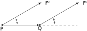
In Section 11.8, we learned how add and subtract vectors and how to multiply vectors by scalars. In this section, we define a product of vectors. We begin with the following definition.

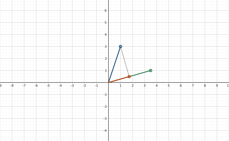
Interactive figureThe dot product builds the shadow: proj_w(v) = (v·w / w·w) wDrag the 4 sliders below the figure.

XYZ Graph · viewer build 5edf91b

Two vectors v = (a, b) and w = (c, d) start at the origin. The rust vector is the projection of v onto w, whose length and direction come entirely from two dot products: proj_w(v) = ((v·w)/(w·w)) w. The dashed segment from the tip of v to the tip of the projection is perpendicular to w, which is the defining property of a projection. Slide the components of either vector: when v and w point the same way the projection is all of v, when they are perpendicular it collapses to the origin, and when the angle between them is obtuse the projection points backwards along w.

Definition

Suppose $\vec{v}$ and $\vec{w}$ are vectors whose component forms are $vector v equals ⟨ v sub 1, v sub 2 ⟩$ and $vector w equals ⟨ w sub 1, w sub 2 ⟩$ . The dot product of $\vec{v}$ and $\vec{w}$ is given by

$\vec{v} \cdot \vec{w} = ⟨ v_{1}, v_{2} ⟩ \cdot ⟨ w_{1}, w_{2} ⟩ = v_{1} w_{1} + v_{2} w_{2}$

For example, let $vector v equals ⟨ 3, 4 ⟩$ and $\vec{w} = ⟨ 1, - 2 ⟩$ . Then $\vec{v} \cdot \vec{w} = ⟨ 3, 4 ⟩ \cdot ⟨ 1, - 2 ⟩ = (3) (1) + (4) (- 2) = - 5$ . Note that the dot product takes two vectors and produces a scalar. For that reason, the quantity $\vec{v} \cdot \vec{w}$ is often called the scalar product of $\vec{v}$ and $\vec{w}$ . The dot product enjoys the following properties.

Theorem

Properties of the Dot Product

Commutative Property: For all vectors $\vec{v}$ and $\vec{w}$ , $\vec{v} \cdot \vec{w} = \vec{w} \cdot \vec{v}$ .
Distributive Property: For all vectors $\vec{u}$ , $\vec{v}$ and $\vec{w}$ , $\vec{u} \cdot (\vec{v} + \vec{w}) = \vec{u} \cdot \vec{v} + \vec{u} \cdot \vec{w}$ .
Scalar Property: For all vectors $\vec{v}$ and $\vec{w}$ and scalars $k$ , $(k \vec{v}) \cdot \vec{w} = k (\vec{v} \cdot \vec{w}) = \vec{v} \cdot (k \vec{w})$ .
Relation to Magnitude: For all vectors $\vec{v}$ , $\vec{v} \cdot \vec{v} = {‖ \vec{v} ‖}^{2}$ .

Like most of the theorems involving vectors, the proof of Theorem 11.22 amounts to using the definition of the dot product and properties of real number arithmetic. To show the commutative property for instance, let $vector v equals ⟨ v sub 1, v sub 2 ⟩$ and $vector w equals ⟨ w sub 1, w sub 2 ⟩$ . Then

$\begin{matrix} \vec{v} \cdot \vec{w} & = & ⟨ v_{1}, v_{2} ⟩ \cdot ⟨ w_{1}, w_{2} ⟩ \\ = & v_{1} w_{1} + v_{2} w_{2} & Definition of Dot Product \\ = & w_{1} v_{1} + w_{2} v_{2} & Commutativity of Real Number Multiplication \\ = & ⟨ w_{1}, w_{2} ⟩ \cdot ⟨ v_{1}, v_{2} ⟩ & Definition of Dot Product \\ = & \vec{w} \cdot \vec{v} \end{matrix}$

The distributive property is proved similarly and is left as an exercise.

For the scalar property, assume that $vector v equals ⟨ v sub 1, v sub 2 ⟩$ and $vector w equals ⟨ w sub 1, w sub 2 ⟩$ and $k$ is a scalar. Then

$\begin{matrix} (k \vec{v}) \cdot \vec{w} & = & (k ⟨ v_{1}, v_{2} ⟩) \cdot ⟨ w_{1}, w_{2} ⟩ \\ = & ⟨ k v_{1}, k v_{2} ⟩ \cdot ⟨ w_{1}, w_{2} ⟩ & Definition of Scalar Multiplication \\ = & (k v_{1}) (w_{1}) + (k v_{2}) (w_{2}) & Definition of Dot Product \\ = & k (v_{1} w_{1}) + k (v_{2} w_{2}) & Associativity of Real Number Multiplication \\ = & k (v_{1} w_{1} + v_{2} w_{2}) & Distributive Law of Real Numbers \\ = & k ⟨ v_{1}, v_{2} ⟩ \cdot ⟨ w_{1}, w_{2} ⟩ & Definition of Dot Product \\ = & k (\vec{v} \cdot \vec{w}) \end{matrix}$

We leave the proof of $k (\vec{v} \cdot \vec{w}) = \vec{v} \cdot (k \vec{w})$ as an exercise.

For the last property, we note that if $vector v equals ⟨ v sub 1, v sub 2 ⟩$ , then $\vec{v} \cdot \vec{v} = ⟨ v_{1}, v_{2} ⟩ \cdot ⟨ v_{1}, v_{2} ⟩ = v_{1}^{2} + v_{2}^{2} = {‖ \vec{v} ‖}^{2}$ , where the last equality comes courtesy of Definition 11.8.

The following example puts Theorem 11.22 to good use. As in Example 11.8.3, we work out the problem in great detail and encourage the reader to supply the justification for each step.

Example 1

Prove the identity: ${‖ \vec{v} - \vec{w} ‖}^{2} = {‖ \vec{v} ‖}^{2} - 2 (\vec{v} \cdot \vec{w}) + {‖ \vec{w} ‖}^{2}$ .

We begin by rewriting ${‖ \vec{v} - \vec{w} ‖}^{2}$ in terms of the dot product using Theorem 11.22.

$\begin{matrix} {‖ \vec{v} - \vec{w} ‖}^{2} & = & (\vec{v} - \vec{w}) \cdot (\vec{v} - \vec{w}) \\ = & (\vec{v} + [- \vec{w}]) \cdot (\vec{v} + [- \vec{w}]) \\ = & (\vec{v} + [- \vec{w}]) \cdot \vec{v} + (\vec{v} + [- \vec{w}]) \cdot [- \vec{w}] \\ = & \vec{v} \cdot (\vec{v} + [- \vec{w}]) + [- \vec{w}] \cdot (\vec{v} + [- \vec{w}]) \\ = & \vec{v} \cdot \vec{v} + \vec{v} \cdot [- \vec{w}] + [- \vec{w}] \cdot \vec{v} + [- \vec{w}] \cdot [- \vec{w}] \\ = & \vec{v} \cdot \vec{v} + \vec{v} \cdot [(- 1) \vec{w}] + [(- 1) \vec{w}] \cdot \vec{v} + [(- 1) \vec{w}] \cdot [(- 1) \vec{w}] \\ = & \vec{v} \cdot \vec{v} + (- 1) (\vec{v} \cdot \vec{w}) + (- 1) (\vec{w} \cdot \vec{v}) + [(- 1) (- 1)] (\vec{w} \cdot \vec{w}) \\ = & \vec{v} \cdot \vec{v} + (- 1) (\vec{v} \cdot \vec{w}) + (- 1) (\vec{v} \cdot \vec{w}) + \vec{w} \cdot \vec{w} \\ = & \vec{v} \cdot \vec{v} - 2 (\vec{v} \cdot \vec{w}) + \vec{w} \cdot \vec{w} \\ = & {‖ \vec{v} ‖}^{2} - 2 (\vec{v} \cdot \vec{w}) + {‖ \vec{w} ‖}^{2} \end{matrix}$

Hence, ${‖ \vec{v} - \vec{w} ‖}^{2} = {‖ \vec{v} ‖}^{2} - 2 (\vec{v} \cdot \vec{w}) + {‖ \vec{w} ‖}^{2}$ as required.

If we take a step back from the pedantry in Example 11.9.1, we see that the bulk of the work is needed to show that $(\vec{v} - \vec{w}) \cdot (\vec{v} - \vec{w}) = \vec{v} \cdot \vec{v} - 2 (\vec{v} \cdot \vec{w}) + \vec{w} \cdot \vec{w}$ . If this looks familiar, it should. Since the dot product enjoys many of the same properties enjoyed by real numbers, the machinations required to expand $(\vec{v} - \vec{w}) \cdot (\vec{v} - \vec{w})$ for vectors $\vec{v}$ and $\vec{w}$ match those required to expand $(v - w) (v - w)$ for real numbers $v$ and $w$ , and hence we get similar looking results. The identity verified in Example 11.9.1 plays a large role in the development of the geometric properties of the dot product, which we now explore.

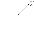
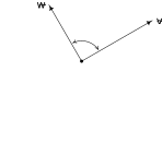
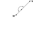
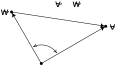
Suppose $\vec{v}$ and $\vec{w}$ are two nonzero vectors. If we draw $\vec{v}$ and $\vec{w}$ with the same initial point, we define the angle between $\vec{v}$ and $\vec{w}$ to be the angle $θ$ determined by the rays containing the vectors $\vec{v}$ and $\vec{w}$ , as illustrated below. We require $0 less than or equal to θ less than or equal to π$ . (Think about why this is needed in the definition.)

Coordinate-plane figure. — **Figure 11.278**

$θ equals 0$

$0 less than θ less than π$

$θ = π$

The following theorem gives us some insight into the geometric role the dot product plays.

Theorem

Geometric Interpretation of Dot Product: If $\vec{v}$ and $\vec{w}$ are nonzero vectors then $\vec{v} \cdot \vec{w} = ‖ \vec{v} ‖ ‖ \vec{w} ‖ \cos (θ)$ , where $θ$ is the angle between $\vec{v}$ and $\vec{w}$ .

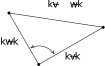
We prove Theorem 11.23 in cases. If $θ equals 0$ , then $\vec{v}$ and $\vec{w}$ have the same direction. It follows¹ that there is a real number $k greater than 0$ so that $\vec{w} = k \vec{v}$ . Hence, $\vec{v} \cdot \vec{w} = \vec{v} \cdot (k \vec{v}) = k (\vec{v} \cdot \vec{v}) = k {‖ \vec{v} ‖}^{2} = k ‖ \vec{v} ‖ ‖ \vec{v} ‖$ . Since $k greater than 0$ , $k = | k |$ , so $k ‖ \vec{v} ‖ = | k | ‖ \vec{v} ‖ = ‖ k \vec{v} ‖$ by Theorem 11.20. Hence, $k ‖ \vec{v} ‖ ‖ \vec{v} ‖ = ‖ \vec{v} ‖ (k ‖ \vec{v} ‖) = ‖ \vec{v} ‖ ‖ k \vec{v} ‖ = ‖ \vec{v} ‖ ‖ \vec{w} ‖$ . Since $cos ⁡ open parenthesis 0 close parenthesis equals 1$ , we get $\vec{v} \cdot \vec{w} = k ‖ \vec{v} ‖ ‖ \vec{v} ‖ = ‖ \vec{v} ‖ ‖ \vec{w} ‖ = ‖ \vec{v} ‖ ‖ \vec{w} ‖ \cos (0)$ , proving that the formula holds for $θ equals 0$ . If $θ = π$ , we repeat the argument with the difference being $\vec{w} = k \vec{v}$ where $k less than 0$ . In this case, $| k | = - k$ , so $k ‖ \vec{v} ‖ = - | k | ‖ \vec{v} ‖ = - ‖ k \vec{v} ‖ = - ‖ \vec{w} ‖$ . Since $\cos (π) = - 1$ , we get $\vec{v} \cdot \vec{w} = - ‖ \vec{v} ‖ ‖ \vec{w} ‖ = ‖ \vec{v} ‖ ‖ \vec{w} ‖ \cos (π)$ , as required. Next, if $0 less than θ less than π$ , the vectors $\vec{v}$ , $\vec{w}$ and $\vec{v} - \vec{w}$ determine a triangle with side lengths $‖ \vec{v} ‖$ , $‖ \vec{w} ‖$ and $‖ \vec{v} - \vec{w} ‖$ , respectively, as seen below.

The Law of Cosines yields ${‖ \vec{v} - \vec{w} ‖}^{2} = {‖ \vec{v} ‖}^{2} + {‖ \vec{w} ‖}^{2} - 2 ‖ \vec{v} ‖ ‖ \vec{w} ‖ \cos (θ)$ . From Example 11.9.1, we know ${‖ \vec{v} - \vec{w} ‖}^{2} = {‖ \vec{v} ‖}^{2} - 2 (\vec{v} \cdot \vec{w}) + {‖ \vec{w} ‖}^{2}$ . Equating these two expressions for ${‖ \vec{v} - \vec{w} ‖}^{2}$ gives ${‖ \vec{v} ‖}^{2} + {‖ \vec{w} ‖}^{2} - 2 ‖ \vec{v} ‖ ‖ \vec{w} ‖ \cos (θ) = {‖ \vec{v} ‖}^{2} - 2 (\vec{v} \cdot \vec{w}) + {‖ \vec{w} ‖}^{2}$ which reduces to $- 2 ‖ \vec{v} ‖ ‖ \vec{w} ‖ \cos (θ) = - 2 (\vec{v} \cdot \vec{w})$ , or $\vec{v} \cdot \vec{w} = ‖ \vec{v} ‖ ‖ \vec{w} ‖ \cos (θ)$ , as required. An immediate consequence of Theorem 11.23 is the following.

Theorem

Let $\vec{v}$ and $\vec{w}$ be nonzero vectors and let $θ$ the angle between $\vec{v}$ and $\vec{w}$ . Then

$θ = \arccos (\frac{\vec{v} \cdot \vec{w}}{‖ \vec{v} ‖ ‖ \vec{w} ‖}) = \arccos (\hat{v} \cdot \hat{w})$

We obtain the formula in Theorem 11.24 by solving the equation given in Theorem 11.23 for $θ$ . Since $\vec{v}$ and $\vec{w}$ are nonzero, so are $‖ \vec{v} ‖$ and $‖ \vec{w} ‖$ . Hence, we may divide both sides of $\vec{v} \cdot \vec{w} = ‖ \vec{v} ‖ ‖ \vec{w} ‖ \cos (θ)$ by $‖ \vec{v} ‖ ‖ \vec{w} ‖$ to get $\cos (θ) = \frac{\vec{v} \cdot \vec{w}}{‖ \vec{v} ‖ ‖ \vec{w} ‖}$ . Since $0 less than or equal to θ less than or equal to π$ by definition, the values of $θ$ exactly match the range of the arccosine function. Hence, $θ = \arccos (\frac{\vec{v} \cdot \vec{w}}{‖ \vec{v} ‖ ‖ \vec{w} ‖})$ . Using Theorem 11.22, we can rewrite $\frac{\vec{v} \cdot \vec{w}}{‖ \vec{v} ‖ ‖ \vec{w} ‖} = (\frac{1}{‖ \vec{v} ‖} \vec{v}) \cdot (\frac{1}{‖ \vec{w} ‖} \vec{w}) = \hat{v} \cdot \hat{w}$ , giving us the alternative formula $θ = \arccos (\hat{v} \cdot \hat{w})$ .

We are overdue for an example.

Example 2

Find the angle between the following pairs of vectors.

$\vec{v} = ⟨ 3, - 3 \sqrt{3} ⟩$ , and $\vec{w} = ⟨ - \sqrt{3}, 1 ⟩$
$vector v equals ⟨ 2, 2 ⟩$ , and $\vec{w} = ⟨ 5, - 5 ⟩$
$\vec{v} = ⟨ 3, - 4 ⟩$ , and $vector w equals ⟨ 2, 1 ⟩$

We use the formula $θ = \arccos (\frac{\vec{v} \cdot \vec{w}}{‖ \vec{v} ‖ ‖ \vec{w} ‖})$ from Theorem 11.24 in each case below.

We have $\vec{v} \cdot \vec{w} = ⟨ 3, - 3 \sqrt{3} ⟩ \cdot ⟨ - \sqrt{3}, 1 ⟩ = - 3 \sqrt{3} - 3 \sqrt{3} = - 6 \sqrt{3}$ . Since $‖ \vec{v} ‖ = \sqrt{3^{2} + {(- 3 \sqrt{3})}^{2}} = \sqrt{36} = 6$ and $‖ \vec{w} ‖ = \sqrt{{(- \sqrt{3})}^{2} + 1^{2}} = \sqrt{4} = 2$ , $θ = \arccos (\frac{- 6 \sqrt{3}}{12}) = \arccos (- \frac{\sqrt{3}}{2}) = \frac{5 π}{6}$ .
For $vector v equals ⟨ 2, 2 ⟩$ and $\vec{w} = ⟨ 5, - 5 ⟩$ , we find $\vec{v} \cdot \vec{w} = ⟨ 2, 2 ⟩ \cdot ⟨ 5, - 5 ⟩ = 10 - 10 = 0$ . Hence, it doesn't matter what $‖ \vec{v} ‖$ and $‖ \vec{w} ‖$ are,² $θ = \arccos (\frac{\vec{v} \cdot \vec{w}}{‖ \vec{v} ‖ ‖ \vec{w} ‖}) = \arccos (0) = \frac{π}{2}$ .
We find $\vec{v} \cdot \vec{w} = ⟨ 3, - 4 ⟩ \cdot ⟨ 2, 1 ⟩ = 6 - 4 = 2$ . Also $‖ \vec{v} ‖ = \sqrt{3^{2} + {(- 4)}^{2}} = \sqrt{25} = 5$ and $\vec{w} = \sqrt{2^{2} + 1^{2}} = \sqrt{5}$ , so $θ = \arccos (\frac{2}{5 \sqrt{5}}) = \arccos (\frac{2 \sqrt{5}}{25})$ . Since $\frac{2 \sqrt{5}}{25}$ isn't the cosine of one of the common angles, we leave our answer as $θ = \arccos (\frac{2 \sqrt{5}}{25})$ .

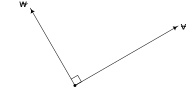
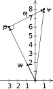
The vectors $vector v equals ⟨ 2, 2 ⟩$ , and $\vec{w} = ⟨ 5, - 5 ⟩$ in Example 11.9.2 are called orthogonal and we write $\vec{v} ⟂ \vec{w}$ , because the angle between them is $\frac{π}{2} radians = 90^{\circ}$ . Geometrically, when orthogonal vectors are sketched with the same initial point, the lines containing the vectors are perpendicular.

$\vec{v}$ and $\vec{w}$ are orthogonal, $\vec{v} ⟂ \vec{w}$

We state the relationship between orthogonal vectors and their dot product in the following theorem.

To prove Theorem 11.25, we first assume $\vec{v}$ and $\vec{w}$ are nonzero vectors with $\vec{v} ⟂ \vec{w}$ . By definition, the angle between $\vec{v}$ and $\vec{w}$ is $\frac{π}{2}$ . By Theorem 11.23, $\vec{v} \cdot \vec{w} = ‖ \vec{v} ‖ ‖ \vec{w} ‖ \cos (\frac{π}{2}) = 0$ . Conversely, if $\vec{v}$ and $\vec{w}$ are nonzero vectors and $\vec{v} \cdot \vec{w} = 0$ , then Theorem 11.24 gives $θ = \arccos (\frac{\vec{v} \cdot \vec{w}}{‖ \vec{v} ‖ ‖ \vec{w} ‖}) = \arccos (\frac{0}{‖ \vec{v} ‖ ‖ \vec{w} ‖}) = \arccos (0) = \frac{π}{2}$ , so $\vec{v} ⟂ \vec{w}$ . We can use Theorem 11.25 in the following example to provide a different proof about the relationship between the slopes of perpendicular lines.³

Example 3

Let $L sub 1$ be the line $y = m_{1} x + b_{1}$ and let $L sub 2$ be the line $y = m_{2} x + b_{2}$ . Prove that $L sub 1$ is perpendicular to $L sub 2$ if and only if $m_{1} \cdot m_{2} = - 1$ .

Our strategy is to find two vectors: $vector v sub 1$ , which has the same direction as $L sub 1$ , and $vector v sub 2$ , which has the same direction as $L sub 2$ and show $vector v sub 1 ⟂ vector v sub 2$ if and only if $m_{1} m_{2} = - 1$ . To that end, we substitute $x equals 0$ and $x equals 1$ into $y = m_{1} x + b_{1}$ to find two points which lie on $L sub 1$ , namely $P ⁢ open parenthesis 0, b sub 1 close parenthesis$ and $Q ⁢ open parenthesis 1, m sub 1 plus b sub 1 close parenthesis$ . We let $\vec{v_{1}} = \vec{P Q} = ⟨ 1 - 0, (m_{1} + b_{1}) - b_{1} ⟩ = ⟨ 1, m_{1} ⟩$ , and note that since $vector v sub 1$ is determined by two points on $L sub 1$ , it may be viewed as lying on $L sub 1$ . Hence it has the same direction as $L sub 1$ . Similarly, we get the vector $vector v sub 2 equals ⟨ 1, m sub 2 ⟩$ which has the same direction as the line $L sub 2$ . Hence, $L sub 1$ and $L sub 2$ are perpendicular if and only if $vector v sub 1 ⟂ vector v sub 2$ . According to Theorem 11.25, $vector v sub 1 ⟂ vector v sub 2$ if and only if $\vec{v_{1}} \cdot \vec{v_{2}} = 0$ . Notice that $\vec{v_{1}} \cdot \vec{v_{2}} = ⟨ 1, m_{1} ⟩ \cdot ⟨ 1, m_{2} ⟩ = 1 + m_{1} m_{2}$ . Hence, $\vec{v_{1}} \cdot \vec{v_{2}} = 0$ if and only if $1 + m_{1} m_{2} = 0$ , which is true if and only if $m_{1} m_{2} = - 1$ , as required.

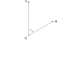
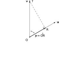
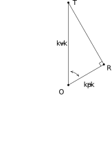
While Theorem 11.25 certainly gives us some insight into what the dot product means geometrically, there is more to the story of the dot product. Consider the two nonzero vectors $\vec{v}$ and $\vec{w}$ drawn with a common initial point $O$ below. For the moment, assume that the angle between $\vec{v}$ and $\vec{w}$ , which we'll denote $θ$ , is acute. We wish to develop a formula for the vector $\vec{p}$ , indicated below, which is called the orthogonal projection of $\vec{v}$ onto $\vec{w}$ . The vector $\vec{p}$ is obtained geometrically as follows: drop a perpendicular from the terminal point $T$ of $\vec{v}$ to the vector $\vec{w}$ and call the point of intersection $R$ . The vector $\vec{p}$ is then defined as $\vec{p} = \vec{O R}$ . Like any vector, $\vec{p}$ is determined by its magnitude $‖ \vec{p} ‖$ and its direction $\hat{p}$ according to the formula $\vec{p} = ‖ \vec{p} ‖ \hat{p}$ . Since we want $\hat{p}$ to have the same direction as $\vec{w}$ , we have $\hat{p} = \hat{w}$ . To determine $‖ \vec{p} ‖$ , we make use of Theorem 10.4 as applied to the right triangle $△ O R T$ . We find $\cos (θ) = \frac{‖ \vec{p} ‖}{‖ \vec{v} ‖}$ , or $‖ \vec{p} ‖ = ‖ \vec{v} ‖ \cos (θ)$ . To get things in terms of just $\vec{v}$ and $\vec{w}$ , we use Theorem 11.23 to get $‖ \vec{p} ‖ = ‖ \vec{v} ‖ \cos (θ) = \frac{‖ \vec{v} ‖ ‖ \vec{w} ‖ \cos (θ)}{‖ \vec{w} ‖} = \frac{\vec{v} \cdot \vec{w}}{‖ \vec{w} ‖}$ . Using Theorem 11.22, we rewrite $\frac{\vec{v} \cdot \vec{w}}{‖ \vec{w} ‖} = \vec{v} \cdot (\frac{1}{‖ \vec{w} ‖} \vec{w}) = \vec{v} \cdot \hat{w}$ . Hence, $‖ \vec{p} ‖ = \vec{v} \cdot \hat{w}$ , and since $\hat{p} = \hat{w}$ , we now have a formula for $\vec{p}$ completely in terms of $\vec{v}$ and $\vec{w}$ , namely $\vec{p} = ‖ \vec{p} ‖ \hat{p} = (\vec{v} \cdot \hat{w}) \hat{w}$ .

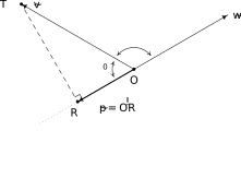
Now suppose that the angle $θ$ between $\vec{v}$ and $\vec{w}$ is obtuse, and consider the diagram below. In this case, we see that $\hat{p} = - \hat{w}$ and using the triangle $△ O R T$ , we find $‖ \vec{p} ‖ = ‖ \vec{v} ‖ \cos (θ^{'})$ . Since $θ + θ^{'} = π$ , it follows that $\cos (θ^{'}) = - \cos (θ)$ , which means $‖ \vec{p} ‖ = ‖ \vec{v} ‖ \cos (θ^{'}) = - ‖ \vec{v} ‖ \cos (θ)$ . Rewriting this last equation in terms of $\vec{v}$ and $\vec{w}$ as before, we get $‖ \vec{p} ‖ = - (\vec{v} \cdot \hat{w})$ . Putting this together with $\hat{p} = - \hat{w}$ , we get $\vec{p} = ‖ \vec{p} ‖ \hat{p} = - (\vec{v} \cdot \hat{w}) (- \hat{w}) = (\vec{v} \cdot \hat{w}) \hat{w}$ in this case as well.

If the angle between $\vec{v}$ and $\vec{w}$ is $\frac{π}{2}$ then it is easy to show⁴ that $vector p equals vector 0$ . Since $\vec{v} ⟂ \vec{w}$ in this case, $\vec{v} \cdot \vec{w} = 0$ . It follows that $\vec{v} \cdot \hat{w} = 0$ and $\vec{p} = \vec{0} = 0 \hat{w} = (\vec{v} \cdot \hat{w}) \hat{w}$ in this case, too. This gives us

Definition

Let $\vec{v}$ and $\vec{w}$ be nonzero vectors. The orthogonal projection of $\vec{v}$ onto $\vec{w}$ , denoted ${proj}_{\vec{w}} (\vec{v})$ is given by ${proj}_{\vec{w}} (\vec{v}) = (\vec{v} \cdot \hat{w}) \hat{w}$ .

Definition 11.12 gives us a good idea what the dot product does. The scalar $\vec{v} \cdot \hat{w}$ is a measure of how much of the vector $\vec{v}$ is in the direction of the vector $\vec{w}$ and is thus called the scalar projection of $\vec{v}$ onto $\vec{w}$ . While the formula given in Definition 11.12 is theoretically appealing, because of the presence of the normalized unit vector $\hat{w}$ , computing the projection using the formula ${proj}_{\vec{w}} (\vec{v}) = (\vec{v} \cdot \hat{w}) \hat{w}$ can be messy. We present two other formulas that are often used in practice.

Theorem

Alternate Formulas for Vector Projections: If $\vec{v}$ and $\vec{w}$ are nonzero vectors then

${proj}_{\vec{w}} (\vec{v}) = (\vec{v} \cdot \hat{w}) \hat{w} = (\frac{\vec{v} \cdot \vec{w}}{{‖ \vec{w} ‖}^{2}}) \vec{w} = (\frac{\vec{v} \cdot \vec{w}}{\vec{w} \cdot \vec{w}}) \vec{w}$

The proof of Theorem 11.26, which we leave to the reader as an exercise, amounts to using the formula $\hat{w} = (\frac{1}{‖ \vec{w} ‖}) \vec{w}$ and properties of the dot product. It is time for an example.

Example 4

Let $vector v equals ⟨ 1, 8 ⟩$ and $\vec{w} = ⟨ - 1, 2 ⟩$ . Find $\vec{p} = {proj}_{\vec{w}} (\vec{v})$ , and plot $\vec{v}$ , $\vec{w}$ and $\vec{p}$ in standard position.

We find $\vec{v} \cdot \vec{w} = ⟨ 1, 8 ⟩ \cdot ⟨ - 1, 2 ⟩ = (- 1) + 16 = 15$ and $\vec{w} \cdot \vec{w} = ⟨ - 1, 2 ⟩ \cdot ⟨ - 1, 2 ⟩ = 1 + 4 = 5$ . Hence, $\vec{p} = \frac{\vec{v} \cdot \vec{w}}{\vec{w} \cdot \vec{w}} \vec{w} = \frac{15}{5} ⟨ - 1, 2 ⟩ = ⟨ - 3, 6 ⟩$ . We plot $\vec{v}$ , $\vec{w}$ and $\vec{p}$ below.

Figure 11.288

Suppose we wanted to verify that our answer $\vec{p}$ in Example 11.9.4 is indeed the orthogonal projection of $\vec{v}$ onto $\vec{w}$ . We first note that since $\vec{p}$ is a scalar multiple of $\vec{w}$ , it has the correct direction, so what remains to check is the orthogonality condition. Consider the vector $\vec{q}$ whose initial point is the terminal point of $\vec{p}$ and whose terminal point is the terminal point of $\vec{v}$ .

From the definition of vector arithmetic, $\vec{p} + \vec{q} = \vec{v}$ , so that $\vec{q} = \vec{v} - \vec{p}$ . In the case of Example 11.9.4, $vector v equals ⟨ 1, 8 ⟩$ and $\vec{p} = ⟨ - 3, 6 ⟩$ , so $\vec{q} = ⟨ 1, 8 ⟩ - ⟨ - 3, 6 ⟩ = ⟨ 4, 2 ⟩$ . Then $\vec{q} \cdot \vec{w} = ⟨ 4, 2 ⟩ \cdot ⟨ - 1, 2 ⟩ = (- 4) + 4 = 0$ , which shows $\vec{q} ⟂ \vec{w}$ , as required. This result is generalized in the following theorem.

Theorem

Generalized Decomposition Theorem: Let $\vec{v}$ and $\vec{w}$ be nonzero vectors. There are unique vectors $\vec{p}$ and $\vec{q}$ such that $\vec{v} = \vec{p} + \vec{q}$ where $\vec{p} = k \vec{w}$ for some scalar $k$ , and $\vec{q} \cdot \vec{w} = 0$ .

Note that if the vectors $\vec{p}$ and $\vec{q}$ in Theorem 11.27 are nonzero, then we can say $\vec{p}$ is parallel ⁵ to $\vec{w}$ and $\vec{q}$ is orthogonal to $\vec{w}$ . In this case, the vector $\vec{p}$ is sometimes called the `vector component of $\vec{v}$ parallel to $\vec{w}$ ' and $\vec{q}$ is called the `vector component of $\vec{v}$ orthogonal to $\vec{w}$ .' To prove Theorem 11.27, we take $\vec{p} = {proj}_{\vec{w}} (\vec{v})$ and $\vec{q} = \vec{v} - \vec{p}$ . Then $\vec{p}$ is, by definition, a scalar multiple of $\vec{w}$ . Next, we compute $\vec{q} \cdot \vec{w}$ .

$\begin{matrix} \vec{q} \cdot \vec{w} & = & (\vec{v} - \vec{p}) \cdot \vec{w} & Definition of \vec{q} . \\ = & \vec{v} \cdot \vec{w} - \vec{p} \cdot \vec{w} & Properties of Dot Product \\ = & \vec{v} \cdot \vec{w} - (\frac{\vec{v} \cdot \vec{w}}{\vec{w} \cdot \vec{w}} \vec{w}) \cdot \vec{w} & Since \vec{p} = {proj}_{\vec{w}} (\vec{v}) . \\ = & \vec{v} \cdot \vec{w} - (\frac{\vec{v} \cdot \vec{w}}{\vec{w} \cdot \vec{w}}) (\vec{w} \cdot \vec{w}) & Properties of Dot Product. \\ = & \vec{v} \cdot \vec{w} - \vec{v} \cdot \vec{w} \\ = & 0 \end{matrix}$

Hence, $\vec{q} \cdot \vec{w} = 0$ , as required. At this point, we have shown that the vectors $\vec{p}$ and $\vec{q}$ guaranteed by Theorem 11.27 exist. Now we need to show that they are unique. Suppose $\vec{v} = \vec{p} + \vec{q} = {\vec{p}}^{'} + {\vec{q}}^{'}$ where the vectors ${\vec{p}}^{'}$ and ${\vec{q}}^{'}$ satisfy the same properties described in Theorem 11.27 as $\vec{p}$ and $\vec{q}$ . Then $\vec{p} - {\vec{p}}^{'} = {\vec{q}}^{'} - \vec{q}$ , so $\vec{w} \cdot (\vec{p} - {\vec{p}}^{'}) = \vec{w} \cdot ({\vec{q}}^{'} - \vec{q}) = \vec{w} \cdot {\vec{q}}^{'} - \vec{w} \cdot \vec{q} = 0 - 0 = 0$ . Hence, $\vec{w} \cdot (\vec{p} - {\vec{p}}^{'}) = 0$ . Now there are scalars $k$ and $k^{'}$ so that $\vec{p} = k \vec{w}$ and ${\vec{p}}^{'} = k^{'} \vec{w}$ . This means $\vec{w} \cdot (\vec{p} - {\vec{p}}^{'}) = \vec{w} \cdot (k \vec{w} - k^{'} \vec{w}) = \vec{w} \cdot ([k - k^{'}] \vec{w}) = (k - k^{'}) (\vec{w} \cdot \vec{w}) = (k - k^{'}) {‖ \vec{w} ‖}^{2}$ . Since $vector w not equal to vector 0$ , $‖ vector w ‖ squared not equal to 0$ , which means the only way $\vec{w} \cdot (\vec{p} - {\vec{p}}^{'}) = (k - k^{'}) {‖ \vec{w} ‖}^{2} = 0$ is for $k - k^{'} = 0$ , or $k = k^{'}$ . This means $\vec{p} = k \vec{w} = k^{'} \vec{w} = {\vec{p}}^{'}$ . With ${\vec{q}}^{'} - \vec{q} = \vec{p} - {\vec{p}}^{'} = \vec{p} - \vec{p} = \vec{0}$ , it must be that ${\vec{q}}^{'} = \vec{q}$ as well. Hence, we have shown there is only one way to write $\vec{v}$ as a sum of vectors as described in Theorem 11.27.

We close this section with an application of the dot product. In Physics, if a constant force $F$ is exerted over a distance $d$ , the work $W$ done by the force is given by $W = F d$ . Here, we assume the force is being applied in the direction of the motion. If the force applied is not in the direction of the motion, we can use the dot product to find the work done. Consider the scenario below where the constant force $\vec{F}$ is applied to move an object from the point $P$ to the point $Q$ .

To find the work $W$ done in this scenario, we need to find how much of the force $\vec{F}$ is in the direction of the motion $\vec{P Q}$ . This is precisely what the dot product $\vec{F} \cdot \hat{P Q}$ represents. Since the distance the object travels is $‖ \vec{P Q} ‖$ , we get $W = (\vec{F} \cdot \hat{P Q}) ‖ \vec{P Q} ‖$ . Since $\vec{P Q} = ‖ \vec{P Q} ‖ \hat{P Q}$ , $W = (\vec{F} \cdot \hat{P Q}) ‖ \vec{P Q} ‖ = \vec{F} \cdot (‖ \vec{P Q} ‖ \hat{P Q}) = \vec{F} \cdot \vec{P Q} = ‖ \vec{F} ‖ ‖ \vec{P Q} ‖ \cos (θ)$ , where $θ$ is the angle between the applied force $\vec{F}$ and the trajectory of the motion $\vec{P Q}$ . We have proved the following.

Theorem

Work as a Dot Product: Suppose a constant force $\vec{F}$ is applied along the vector $\vec{P Q}$ . The work $W$ done by $\vec{F}$ is given by

$W = \vec{F} \cdot \vec{P Q} = ‖ \vec{F} ‖ ‖ \vec{P Q} ‖ \cos (θ),$

where $θ$ is the angle between $\vec{F}$ and $\vec{P Q}$ .

Example 5

Taylor exerts a force of $10$ pounds to pull her wagon a distance of $50$ feet over level ground. If the handle of the wagon makes a $30 degrees$ angle with the horizontal, how much work did Taylor do pulling the wagon? Assume Taylor exerts the force of $10$ pounds at a $30 degrees$ angle for the duration of the $50$ feet.

Figure 11.291

There are two ways to attack this problem. One way is to find the vectors $\vec{F}$ and $\vec{P Q}$ mentioned in Theorem 11.28 and compute $W = \vec{F} \cdot \vec{P Q}$ . To do this, we assume the origin is at the point where the handle of the wagon meets the wagon and the positive $x$ -axis lies along the dashed line in the figure above. Since the force applied is a constant 10 pounds, we have $‖ vector F ‖ equals 10$ . Since it is being applied at a constant angle of $θ equals 30 degrees$ with respect to the positive $x$ -axis, Definition 11.8 gives us $\vec{F} = 10 ⟨ \cos (30^{\circ}, \sin (30^{\circ}) ⟩ = ⟨ 5 \sqrt{3}, 5 ⟩$ . Since the wagon is being pulled along 50 feet in the positive direction, the displacement vector is $\vec{P Q} = 50 \hat{ı} = 50 ⟨ 1, 0 ⟩ = ⟨ 50, 0 ⟩$ . We get $W = \vec{F} \cdot \vec{P Q} = ⟨ 5 \sqrt{3}, 5 ⟩ \cdot ⟨ 50, 0 ⟩ = 250 \sqrt{3}$ . Since force is measured in pounds and distance is measured in feet, we get $W = 250 \sqrt{3}$ foot-pounds. Alternatively, we can use the formulation $W = ‖ \vec{F} ‖ ‖ \vec{P Q} ‖ \cos (θ)$ to get $W = (10 pounds) (50 feet) \cos (30^{\circ}) = 250 \sqrt{3}$ foot-pounds of work.

Exercises

In Exercises -, use the pair of vectors $\vec{v}$ and $\vec{w}$ to find the following quantities.

$\vec{v} \cdot \vec{w}$
The angle $θ$ (in degrees) between $\vec{v}$ and $\vec{w}$
${proj}_{\vec{w}} (\vec{v})$
$\vec{q} = \vec{v} - {proj}_{\vec{w}} (\vec{v})$ (Show that $\vec{q} \cdot \vec{w} = 0$ .)

$\vec{v} = ⟨ - 2, - 7 ⟩$ and $\vec{w} = ⟨ 5, - 9 ⟩$
$\vec{v} = ⟨ - 6, - 5 ⟩$ and $\vec{w} = ⟨ 10, - 12 ⟩$
$\vec{v} = ⟨ 1, \sqrt{3} ⟩$ and $\vec{w} = ⟨ 1, - \sqrt{3} ⟩$
$vector v equals ⟨ 3, 4 ⟩$ and $\vec{w} = ⟨ - 6, - 8 ⟩$
$\vec{v} = ⟨ - 2, 1 ⟩$ and $vector w equals ⟨ 3, 6 ⟩$
$\vec{v} = ⟨ - 3 \sqrt{3}, 3 ⟩$ and $\vec{w} = ⟨ - \sqrt{3}, - 1 ⟩$
$vector v equals ⟨ 1, 17 ⟩$ and $\vec{w} = ⟨ - 1, 0 ⟩$
$vector v equals ⟨ 3, 4 ⟩$ and $vector w equals ⟨ 5, 12 ⟩$
$\vec{v} = ⟨ - 4, - 2 ⟩$ and $\vec{w} = ⟨ 1, - 5 ⟩$
$\vec{v} = ⟨ - 5, 6 ⟩$ and $\vec{w} = ⟨ 4, - 7 ⟩$
$\vec{v} = ⟨ - 8, 3 ⟩$ and $vector w equals ⟨ 2, 6 ⟩$
$\vec{v} = ⟨ 34, - 91 ⟩$ and $vector w equals ⟨ 0, 1 ⟩$
$\vec{v} = 3 \hat{ı} - \hat{ȷ}$ and $vector w equals 4 ⁢ ȷ hat$
$\vec{v} = - 24 \hat{ı} + 7 \hat{ȷ}$ and $vector w equals 2 ⁢ ı hat$
$\vec{v} = \frac{3}{2} \hat{ı} + \frac{3}{2} \hat{ȷ}$ and $\vec{w} = \hat{ı} - \hat{ȷ}$
$\vec{v} = 5 \hat{ı} + 12 \hat{ȷ}$ and $\vec{w} = - 3 \hat{ı} + 4 \hat{ȷ}$
$\vec{v} = ⟨ \frac{1}{2}, \frac{\sqrt{3}}{2} ⟩$ and $\vec{w} = ⟨ - \frac{\sqrt{2}}{2}, \frac{\sqrt{2}}{2} ⟩$
$\vec{v} = ⟨ \frac{\sqrt{2}}{2}, \frac{\sqrt{2}}{2} ⟩$ and $\vec{w} = ⟨ \frac{1}{2}, - \frac{\sqrt{3}}{2} ⟩$
$\vec{v} = ⟨ \frac{\sqrt{3}}{2}, \frac{1}{2} ⟩$ and $\vec{w} = ⟨ - \frac{\sqrt{2}}{2}, - \frac{\sqrt{2}}{2} ⟩$
$\vec{v} = ⟨ \frac{1}{2}, - \frac{\sqrt{3}}{2} ⟩$ and $\vec{w} = ⟨ \frac{\sqrt{2}}{2}, - \frac{\sqrt{2}}{2} ⟩$
A force of $1500$ pounds is required to tow a trailer. Find the work done towing the trailer along a flat stretch of road $300$ feet. Assume the force is applied in the direction of the motion.
Find the work done lifting a $10$ pound book $3$ feet straight up into the air. Assume the force of gravity is acting straight downwards.
Suppose Taylor fills her wagon with rocks and must exert a force of 13 pounds to pull her wagon across the yard. If she maintains a $15 degrees$ angle between the handle of the wagon and the horizontal, compute how much work Taylor does pulling her wagon 25 feet. Round your answer to two decimal places.
In Exercise in Section 11.8, two drunken college students have filled an empty beer keg with rocks which they drag down the street by pulling on two attached ropes. The stronger of the two students pulls with a force of 100 pounds on a rope which makes a $13 degrees$ angle with the direction of motion. (In this case, the keg was being pulled due east and the student's heading was N $77 degrees$ E.) Find the work done by this student if the keg is dragged 42 feet.
Find the work done pushing a 200 pound barrel 10 feet up a $12.5 degrees$ incline. Ignore all forces acting on the barrel except gravity, which acts downwards. Round your answer to two decimal places.
HINT: Since you are working to overcome gravity only, the force being applied acts directly upwards. This means that the angle between the applied force in this case and the motion of the object is not the $12.5 degrees$ of the incline!
Prove the distributive property of the dot product in Theorem 11.22.
Finish the proof of the scalar property of the dot product in Theorem 11.22.
Use the identity in Example 11.9.1 to prove the Parallelogram Law
${‖ \vec{v} ‖}^{2} + {‖ \vec{w} ‖}^{2} = \frac{1}{2} [{‖ \vec{v} + \vec{w} ‖}^{2} + {‖ \vec{v} - \vec{w} ‖}^{2}]$
We know that $| x + y | \leq | x | + | y |$ for all real numbers $x$ and $y$ by the Triangle Inequality established in Exercise in Section 2.2. We can now establish a Triangle Inequality for vectors. In this exercise, we prove that $‖ \vec{u} + \vec{v} ‖ \leq ‖ \vec{u} ‖ + ‖ \vec{v} ‖$ for all pairs of vectors $\vec{u}$ and $\vec{v}$ .
1. (Step 1) Show that ${‖ \vec{u} + \vec{v} ‖}^{2} = {‖ \vec{u} ‖}^{2} + 2 \vec{u} \cdot \vec{v} + {‖ \vec{v} ‖}^{2}$ .
2. (Step 2) Show that $| \vec{u} \cdot \vec{v} | \leq ‖ \vec{u} ‖ ‖ \vec{v} ‖$ . This is the celebrated Cauchy-Schwarz Inequality.⁶ (Hint: To show this inequality, start with the fact that $| \vec{u} \cdot \vec{v} | = | ‖ \vec{u} ‖ ‖ \vec{v} ‖ \cos (θ) |$ and use the fact that $vertical bar cos ⁡ open parenthesis θ close parenthesis vertical bar less than or equal to 1$ for all $θ$ .)
3. (Step 3) Show that ${‖ \vec{u} + \vec{v} ‖}^{2} = {‖ \vec{u} ‖}^{2} + 2 \vec{u} \cdot \vec{v} + {‖ \vec{v} ‖}^{2} \leq {‖ \vec{u} ‖}^{2} + 2 | \vec{u} \cdot \vec{v} | + {‖ \vec{v} ‖}^{2} \leq {‖ \vec{u} ‖}^{2} + 2 ‖ \vec{u} ‖ ‖ \vec{v} ‖ + {‖ \vec{v} ‖}^{2} = {(‖ \vec{u} ‖ + ‖ \vec{v} ‖)}^{2}$ .
4. (Step 4) Use Step 3 to show that $‖ \vec{u} + \vec{v} ‖ \leq ‖ \vec{u} ‖ + ‖ \vec{v} ‖$ for all pairs of vectors $\vec{u}$ and $\vec{v}$ .
5. As an added bonus, we can now show that the Triangle Inequality $| z + w | \leq | z | + | w |$ holds for all complex numbers $z$ and $w$ as well. Identify the complex number $z = a + b i$ with the vector $u = ⟨ a, b ⟩$ and identify the complex number $w = c + d i$ with the vector $v = ⟨ c, d ⟩$ and just follow your nose!

Answers

$\vec{v} = ⟨ - 2, - 7 ⟩$ and $\vec{w} = ⟨ 5, - 9 ⟩$
$\vec{v} \cdot \vec{w} = 53$
$θ equals 45 degrees$
${proj}_{\vec{w}} (\vec{v}) = ⟨ \frac{5}{2}, - \frac{9}{2} ⟩$
$\vec{q} = ⟨ - \frac{9}{2}, - \frac{5}{2} ⟩$
$\vec{v} = ⟨ - 6, - 5 ⟩$ and $\vec{w} = ⟨ 10, - 12 ⟩$
$\vec{v} \cdot \vec{w} = 0$
$θ equals 90 degrees$
$proj sub vector w ⁢ open parenthesis vector v close parenthesis equals ⟨ 0, 0 ⟩$
$\vec{q} = ⟨ - 6, - 5 ⟩$
$\vec{v} = ⟨ 1, \sqrt{3} ⟩$ and $\vec{w} = ⟨ 1, - \sqrt{3} ⟩$
$\vec{v} \cdot \vec{w} = - 2$
$θ equals 120 degrees$
${proj}_{\vec{w}} (\vec{v}) = ⟨ - \frac{1}{2}, \frac{\sqrt{3}}{2} ⟩$
$\vec{q} = ⟨ \frac{3}{2}, \frac{\sqrt{3}}{2} ⟩$
$vector v equals ⟨ 3, 4 ⟩$ and $\vec{w} = ⟨ - 6, - 8 ⟩$
$\vec{v} \cdot \vec{w} = - 50$
$θ equals 180 degrees$
$proj sub vector w ⁢ open parenthesis vector v close parenthesis equals ⟨ 3, 4 ⟩$
$vector q equals ⟨ 0, 0 ⟩$
$\vec{v} = ⟨ - 2, 1 ⟩$ and $vector w equals ⟨ 3, 6 ⟩$
$\vec{v} \cdot \vec{w} = 0$
$θ equals 90 degrees$
$proj sub vector w ⁢ open parenthesis vector v close parenthesis equals ⟨ 0, 0 ⟩$
$\vec{q} = ⟨ - 2, 1 ⟩$
$\vec{v} = ⟨ - 3 \sqrt{3}, 3 ⟩$ and $\vec{w} = ⟨ - \sqrt{3}, - 1 ⟩$
$\vec{v} \cdot \vec{w} = 6$
$θ equals 60 degrees$
${proj}_{\vec{w}} (\vec{v}) = ⟨ - \frac{3 \sqrt{3}}{2}, - \frac{3}{2} ⟩$
$\vec{q} = ⟨ - \frac{3 \sqrt{3}}{2}, \frac{9}{2} ⟩$
$vector v equals ⟨ 1, 17 ⟩$ and $\vec{w} = ⟨ - 1, 0 ⟩$
$\vec{v} \cdot \vec{w} = - 1$
$θ approximately equals 93.37 degrees$
$proj sub vector w ⁢ open parenthesis vector v close parenthesis equals ⟨ 1, 0 ⟩$
$vector q equals ⟨ 0, 17 ⟩$
$vector v equals ⟨ 3, 4 ⟩$ and $vector w equals ⟨ 5, 12 ⟩$
$\vec{v} \cdot \vec{w} = 63$
$θ approximately equals 14.25 degrees$
${proj}_{\vec{w}} (\vec{v}) = ⟨ \frac{315}{169}, \frac{756}{169} ⟩$
$\vec{q} = ⟨ \frac{192}{169}, - \frac{80}{169} ⟩$
$\vec{v} = ⟨ - 4, - 2 ⟩$ and $\vec{w} = ⟨ 1, - 5 ⟩$
$\vec{v} \cdot \vec{w} = 6$
$θ approximately equals 74.74 degrees$
${proj}_{\vec{w}} (\vec{v}) = ⟨ \frac{3}{13}, - \frac{15}{13} ⟩$
$\vec{q} = ⟨ - \frac{55}{13}, - \frac{11}{13} ⟩$
$\vec{v} = ⟨ - 5, 6 ⟩$ and $\vec{w} = ⟨ 4, - 7 ⟩$
$\vec{v} \cdot \vec{w} = - 62$
$θ approximately equals 169.94 degrees$
${proj}_{\vec{w}} (\vec{v}) = ⟨ - \frac{248}{65}, \frac{434}{65} ⟩$
$\vec{q} = ⟨ - \frac{77}{65}, - \frac{44}{65} ⟩$
$\vec{v} = ⟨ - 8, 3 ⟩$ and $vector w equals ⟨ 2, 6 ⟩$
$\vec{v} \cdot \vec{w} = 2$
$θ approximately equals 87.88 degrees$
${proj}_{\vec{w}} (\vec{v}) = ⟨ \frac{1}{10}, \frac{3}{10} ⟩$
$\vec{q} = ⟨ - \frac{81}{10}, \frac{27}{10} ⟩$
$\vec{v} = ⟨ 34, - 91 ⟩$ and $vector w equals ⟨ 0, 1 ⟩$
$\vec{v} \cdot \vec{w} = - 91$
$θ approximately equals 159.51 degrees$
${proj}_{\vec{w}} (\vec{v}) = ⟨ 0, - 91 ⟩$
$vector q equals ⟨ 34, 0 ⟩$
$\vec{v} = 3 \hat{ı} - \hat{ȷ}$ and $vector w equals 4 ⁢ ȷ hat$
$\vec{v} \cdot \vec{w} = - 4$
$θ approximately equals 108.43 degrees$
${proj}_{\vec{w}} (\vec{v}) = ⟨ 0, - 1 ⟩$
$vector q equals ⟨ 3, 0 ⟩$
$\vec{v} = - 24 \hat{ı} + 7 \hat{ȷ}$ and $vector w equals 2 ⁢ ı hat$
$\vec{v} \cdot \vec{w} = - 48$
$θ approximately equals 163.74 degrees$
${proj}_{\vec{w}} (\vec{v}) = ⟨ - 24, 0 ⟩$
$vector q equals ⟨ 0, 7 ⟩$
$\vec{v} = \frac{3}{2} \hat{ı} + \frac{3}{2} \hat{ȷ}$ and $\vec{w} = \hat{ı} - \hat{ȷ}$
$\vec{v} \cdot \vec{w} = 0$
$θ equals 90 degrees$
$proj sub vector w ⁢ open parenthesis vector v close parenthesis equals ⟨ 0, 0 ⟩$
$\vec{q} = ⟨ \frac{3}{2}, \frac{3}{2} ⟩$
$\vec{v} = 5 \hat{ı} + 12 \hat{ȷ}$ and $\vec{w} = - 3 \hat{ı} + 4 \hat{ȷ}$
$\vec{v} \cdot \vec{w} = 33$
$θ approximately equals 59.49 degrees$
${proj}_{\vec{w}} (\vec{v}) = ⟨ - \frac{99}{25}, \frac{132}{25} ⟩$
$\vec{q} = ⟨ \frac{224}{25}, \frac{168}{25} ⟩$
$\vec{v} = ⟨ \frac{1}{2}, \frac{\sqrt{3}}{2} ⟩$ and $\vec{w} = ⟨ - \frac{\sqrt{2}}{2}, \frac{\sqrt{2}}{2} ⟩$
$\vec{v} \cdot \vec{w} = \frac{\sqrt{6} - \sqrt{2}}{4}$
$θ equals 75 degrees$
${proj}_{\vec{w}} (\vec{v}) = ⟨ \frac{1 - \sqrt{3}}{4}, \frac{\sqrt{3} - 1}{4} ⟩$
$\vec{q} = ⟨ \frac{1 + \sqrt{3}}{4}, \frac{1 + \sqrt{3}}{4} ⟩$
$\vec{v} = ⟨ \frac{\sqrt{2}}{2}, \frac{\sqrt{2}}{2} ⟩$ and $\vec{w} = ⟨ \frac{1}{2}, - \frac{\sqrt{3}}{2} ⟩$
$\vec{v} \cdot \vec{w} = \frac{\sqrt{2} - \sqrt{6}}{4}$
$θ equals 105 degrees$
${proj}_{\vec{w}} (\vec{v}) = ⟨ \frac{\sqrt{2} - \sqrt{6}}{8}, \frac{3 \sqrt{2} - \sqrt{6}}{8} ⟩$
$\vec{q} = ⟨ \frac{3 \sqrt{2} + \sqrt{6}}{8}, \frac{\sqrt{2} + \sqrt{6}}{8} ⟩$
$\vec{v} = ⟨ \frac{\sqrt{3}}{2}, \frac{1}{2} ⟩$ and $\vec{w} = ⟨ - \frac{\sqrt{2}}{2}, - \frac{\sqrt{2}}{2} ⟩$
$\vec{v} \cdot \vec{w} = - \frac{\sqrt{6} + \sqrt{2}}{4}$
$θ equals 165 degrees$
${proj}_{\vec{w}} (\vec{v}) = ⟨ \frac{\sqrt{3} + 1}{4}, \frac{\sqrt{3} + 1}{4} ⟩$
$\vec{q} = ⟨ \frac{\sqrt{3} - 1}{4}, \frac{1 - \sqrt{3}}{4} ⟩$
$\vec{v} = ⟨ \frac{1}{2}, - \frac{\sqrt{3}}{2} ⟩$ and $\vec{w} = ⟨ \frac{\sqrt{2}}{2}, - \frac{\sqrt{2}}{2} ⟩$
$\vec{v} \cdot \vec{w} = \frac{\sqrt{6} + \sqrt{2}}{4}$
$θ equals 15 degrees$
${proj}_{\vec{w}} (\vec{v}) = ⟨ \frac{\sqrt{3} + 1}{4}, - \frac{\sqrt{3} + 1}{4} ⟩$
$\vec{q} = ⟨ \frac{1 - \sqrt{3}}{4}, \frac{1 - \sqrt{3}}{4} ⟩$
$open parenthesis 1500 ⁢ pounds close parenthesis ⁢ open parenthesis 300 ⁢ feet close parenthesis ⁢ cos ⁡ open parenthesis 0 degrees close parenthesis equals 450, 000$ foot-pounds
$open parenthesis 10 ⁢ pounds close parenthesis ⁢ open parenthesis 3 ⁢ feet close parenthesis ⁢ cos ⁡ open parenthesis 0 degrees close parenthesis equals 30$ foot-pounds
$open parenthesis 13 ⁢ pounds close parenthesis ⁢ open parenthesis 25 ⁢ feet close parenthesis ⁢ cos ⁡ open parenthesis 15 degrees close parenthesis approximately equals 313.92$ foot-pounds
$open parenthesis 100 ⁢ pounds close parenthesis ⁢ open parenthesis 42 ⁢ feet close parenthesis ⁢ cos ⁡ open parenthesis 13 degrees close parenthesis approximately equals 4092.35$ foot-pounds
$open parenthesis 200 ⁢ pounds close parenthesis ⁢ open parenthesis 10 ⁢ feet close parenthesis ⁢ cos ⁡ open parenthesis 77.5 degrees close parenthesis approximately equals 432.88$ foot-pounds

Since $\vec{v} = ‖ \vec{v} ‖ \hat{v}$ and $\vec{w} = ‖ \vec{w} ‖ \hat{w}$ , if $\hat{v} = \hat{w}$ then $\vec{w} = ‖ \vec{w} ‖ \hat{v} = \frac{‖ \vec{w} ‖}{‖ \vec{v} ‖} (‖ \vec{v} ‖ \hat{v}) = \frac{‖ \vec{w} ‖}{‖ \vec{v} ‖} \vec{v}$ . In this case, $k = \frac{‖ \vec{w} ‖}{‖ \vec{v} ‖} > 0$ . ↩
Note that there is no `zero product property' for the dot product since neither $\vec{v}$ nor $\vec{w}$ is $vector 0$ , yet $\vec{v} \cdot \vec{w} = 0$ . ↩
See Exercise in Section 2.1. ↩
In this case, the point $R$ coincides with the point $O$ , so $\vec{p} = \vec{O R} = \vec{O O} = \vec{0}$ . ↩
See Exercise in Section 11.8. ↩
It is also known by other names. Check out this site for details. ↩

Adapted from Precalculus, 3rd corrected edition, by Carl Stitz and Jeff Zeager (stitz-zeager.com), licensed under CC BY-NC-SA 3.0. Changes were made: reformatted as an accessible XYZ web edition. License: CC-BY-NC-SA-3.0.