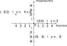
In this section, we return to our study of complex numbers which were first introduced in Section 3.4. Recall that a complex number is a number of the form where and are real numbers and is the imaginary unit defined by . The number is called the real part of , denoted , while the real number is called the imaginary part of , denoted . From Intermediate Algebra, we know that if where , , and are real numbers, then and , which means and are well-defined.1 To start off this section, we associate each complex number with the point on the coordinate plane. In this case, the -axis is relabeled as the real axis, which corresponds to the real number line as usual, and the -axis is relabeled as the imaginary axis, which is demarcated in increments of the imaginary unit . The plane determined by these two axes is called the complex plane.
Figure 11.251
The Complex Plane
Since the ordered pair gives the rectangular coordinates associated with the complex number , the expression is called the rectangular form of . Of course, we could just as easily associate with a pair of polar coordinates . Although it is not as straightforward as the definitions of and , we can still give and special names in relation to .
Some remarks about Definition 11.2 are in order. We know from Section 11.4 that every point in the plane has infinitely many polar coordinate representations which means it's worth our time to make sure the quantities `modulus', `argument' and `principal argument' are well-defined. Concerning the modulus, if then the point associated with is the origin. In this case, the only
-value which can be used here is . Hence for , is well-defined. If , then the point associated with is not the origin, and there are two possibilities for : one positive and one negative. However, we stipulated in our definition so this pins down the value of to one and only one number. Thus the modulus is well-defined in this case, too.2 Even with the requirement , there are infinitely many angles which can be used in a polar representation of a point . If then the point in question is not the origin, so all of these angles are coterminal. Since coterminal angles are exactly radians apart, we are guaranteed that only one of them lies in the interval , and this angle is what we call the principal argument of , . In fact, the set of all arguments of can be described using set-builder notation as . Note that since is a set, we will write `' to mean ` is in3 the set of arguments of '. If then the point in question is the origin, which we know can be represented in polar coordinates as for any angle . In this case, we have and since there is no one value of which lies , we leave undefined.4 It is time for an example.
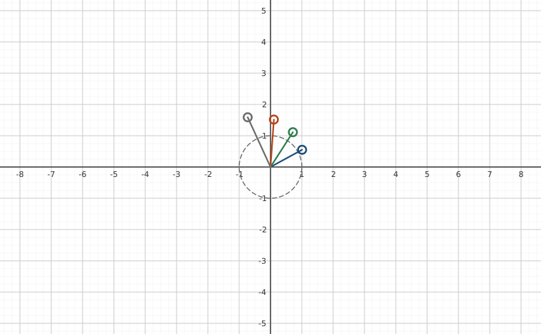
Interactive figureDe Moivre on the complex plane: each power multiplies the modulus and adds the argumentDrag the Modulus r and Argument θ sliders.
XYZ Graph · viewer build 5edf91b
The navy arm is z = r(cos θ + i sin θ) with the modulus and argument on the two sliders; the green, rust and gray arms are z², z³ and z⁴. In polar form powers are easy to see: the modulus goes r, r², r³, r⁴ so the arms lengthen when r > 1 and shrink when r < 1, and the argument goes θ, 2θ, 3θ, 4θ so each arm is turned by one more copy of θ than the last. Set r = 1 and every power stays on the dashed unit circle, marching around it in equal steps, which is the picture behind roots of unity.
Now that we've had some practice computing the modulus and argument of some complex numbers, it is time to explore their properties. We have the following theorem.
To prove the first three properties in Theorem 11.14, suppose where and are real numbers. To determine , we find a polar representation with for the point . From Section 11.4, we know so that . Since we require , then it must be that , which means . Using the distance formula, we find the distance from to is also , establishing the first property.5 For the second property, note that since is a distance, . Furthermore, if and only if the distance from to is , and the latter happens if and only if , which is what we were asked to show.6 For the third property, we note that since and , .
To prove the product rule, suppose and for real numbers , , and . Then . After the usual arithmetic7 we get . Therefore,
Hence as required.
Now that the Product Rule has been established, we use it and the Principle of Mathematical Induction8 to prove the power rule. Let be the statement . Then is true since . Next, assume is true. That is, assume for some . Our job is to show that is true, namely . As is customary with induction proofs, we first try to reduce the problem in such a way as to use the Induction Hypothesis.
Hence, is true, which means is true for all natural numbers .
Like the Power Rule, the Quotient Rule can also be established with the help of the Product Rule. We assume (so ) and we get
Hence, the proof really boils down to showing . This is left as an exercise.
Next, we characterize the argument of a complex number in terms of its real and imaginary parts.
To prove Theorem 11.15, suppose for real numbers and . By definition, and , so the point associated with is . From Section 11.4, we know that if is a polar representation for , then , provided . If and , then lies on the positive imaginary axis. Since we take , we have that is coterminal with , and the result follows. If and , then lies on the negative imaginary axis, and a similar argument shows is coterminal with . The last property in the theorem was already discussed in the remarks following Definition 11.2.
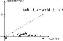
Our next goal is to completely marry the Geometry and the Algebra of the complex numbers. To that end, consider the figure below.
Figure 11.253
Polar coordinates, associated with with .
We know from Theorem 11.7 that and . Making these substitutions for and gives . The expression `' is abbreviated so we can write . Since and , we get
Since there are infinitely many choices for , there infinitely many polar forms for , so we used the indefinite article `a' in Definition 11.3. It is time for an example.
The following theorem summarizes the advantages of working with complex numbers in polar form.
The proof of Theorem 11.16 requires a healthy mix of definition, arithmetic and identities. We first start with the product rule.
We now focus on the quantity in brackets on the right hand side of the equation.
Putting this together with our earlier work, we get , as required.
Moving right along, we next take aim at the Power Rule, better known as DeMoivre's Theorem.9 We proceed by induction on . Let be the sentence . Then is true, since . We now assume is true, that is, we assume for some . Our goal is to show that is true, or that . We have
Hence, assuming is true, we have that is true, so by the Principle of Mathematical Induction, for all natural numbers .
The last property in Theorem 11.16 to prove is the quotient rule. Assuming we have
Next, we multiply both the numerator and denominator of the right hand side by which is the complex conjugate of to get
If we let the numerator be and simplify we get
If we call the denominator then we get
Putting it all together, we get
and we are done. The next example makes good use of Theorem 11.16.
Some remarks are in order. First, the reader may not be sold on using the polar form of complex numbers to multiply complex numbers – especially if they aren't given in polar form to begin with. Indeed, a lot of work was needed to convert the numbers and in Example 11.7.3 into polar form, compute their product, and convert back to rectangular form – certainly more work than is required to multiply out the old-fashioned way. However, Theorem 11.16 pays huge dividends when computing powers of complex numbers. Consider how we computed above and compare that to using the Binomial Theorem, Theorem 9.4, to accomplish the same feat by expanding . Division is tricky in the best of times, and we saved ourselves a lot of time and effort using Theorem 11.16 to find and simplify using their polar forms as opposed to starting with , rationalizing the denominator, and so forth.
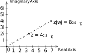
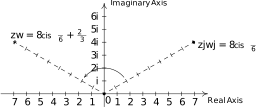
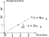
There is geometric reason for studying these polar forms and we would be derelict in our duties if we did not mention the Geometry hidden in Theorem 11.16. Take the product rule, for instance. If and , the formula can be viewed geometrically as a two step process. The multiplication of by can be interpreted as magnifying10 the distance from to , by the factor . Adding the argument of to the argument of can be interpreted geometrically as a rotation of radians counter-clockwise.11 Focusing on and from Example 11.7.3, we can arrive at the product by plotting , doubling its distance from (since ), and rotating radians counter-clockwise. The sequence of diagrams below attempts to describe this process geometrically.
Figure 11.254Figure 11.255
Multiplying by .
Rotating counter-clockwise by radians.
Visualizing for and .
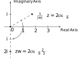
We may also visualize division similarly. Here, the formula may be interpreted as shrinking12 the distance from to by the factor , followed up by a clockwise13 rotation of radians. In the case of and from Example 11.7.3, we arrive at by first halving the distance from to , then rotating clockwise radians.
Figure 11.256Figure 11.257
Dividing by .
Rotating clockwise by radians.
Visualizing for and .
Our last goal of the section is to reverse DeMoivre's Theorem to extract roots of complex numbers.
Unlike Definition 5.4 in Section 5.3, we do not specify one particular prinicpal
root, hence the use of the indefinite article `an' as in `an root of '. Using this definition, both and are square roots of , while means the principal square root of as in . Suppose we wish to find all complex third (cube) roots of . Algebraically, we are trying to solve . We know that there is only one real solution to this equation, namely , but if we take the time to rewrite this equation as and factor, we get . The quadratic factor gives two more cube roots , for a total of three cube roots of . In accordance with Theorem 3.14, since the degree of is three, there are three complex zeros, counting multiplicity. Since we have found three distinct zeros, we know these are all of the zeros, so there are exactly three distinct cube roots of . Let us now solve this same problem using the machinery developed in this section. To do so, we express in polar form. Since lies units away on the positive real axis, we get . If we let be a polar form of , the equation becomes
The complex number on the left hand side of the equation corresponds to the point with polar coordinates , while the complex number on the right hand side corresponds to the point with polar coordinates . Since , so is , which means and are two polar representations corresponding to the same complex number, both with positive values. From Section 11.4, we know and for integers . Since is a real number, we solve by extracting the principal cube root to get . As for , we get for integers . This produces three distinct points with polar coordinates corresponding to , and : specifically , and . These correspond to the complex numbers , and , respectively. Writing these out in rectangular form yields , and . While this process seems a tad more involved than our previous factoring approach, this procedure can be generalized to find, for example, all of the fifth roots of . (Try using Chapter 3 techniques on that!) If we start with a generic complex number in polar form and solve in the same manner as above, we arrive at the following theorem.
The proof of Theorem 11.17 breaks into to two parts: first, showing that each is an root, and second, showing that the set consists of different complex numbers. To show is an root of , we use DeMoivre's Theorem to show .
Since is a whole number, and . Hence, it follows that , so , as required. To show that the formula in Theorem 11.17 generates distinct numbers, we assume (or else there is nothing to prove) and note that the modulus of each of the is the same, namely . Therefore, the only way any two of these polar forms correspond to the same number is if their arguments are coterminal – that is, if the arguments differ by an integer multiple of . Suppose and are whole numbers between and , inclusive, with . Since and are different, let's assume for the sake of argument that . Then . For this to be an integer multiple of , must be a multiple of . But because of the restrictions on and , . (Think this through.) Hence, is a positive number less than , so it cannot be a multiple of . As a result, and are different complex numbers, and we are done. By Theorem 3.14, we know there at most distinct solutions to , and we have just found all of them. We illustrate Theorem 11.17 in the next example.
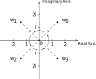
Now that we have done some computations using Theorem 11.17, we take a step back to look at things geometrically. Essentially, Theorem 11.17 says that to find the roots of a complex number, we first take the root of the modulus and divide the argument by . This gives the first root . Each succeessive root is found by adding to the argument, which amounts to rotating by radians. This results in roots, spaced equally around the complex plane. As an example of this, we plot our answers to number in Example 11.7.4 below.
Figure 11.258
The four fourth roots of equally spaced around the plane.
We have only glimpsed at the beauty of the complex numbers in this section. The complex plane is without a doubt one of the most important mathematical constructs ever devised. Coupled with Calculus, it is the venue for incredibly important Science and Engineering applications.14 For now, the following exercises will have to suffice.
Exercises
In Exercises -, find a polar representation for the complex number and then identify , , , and .
In Exercises -, find the rectangular form of the given complex number. Use whatever identities are necessary to find the exact values.
For Exercises -, use and to compute the quantity. Express your answers in polar form using the principal argument.
In Exercises -, use DeMoivre's Theorem to find the indicated power of the given complex number. Express your final answers in rectangular form.
In Exercises -, find the indicated complex roots. Express your answers in polar form and then convert them into rectangular form.
the two square roots of
the two square roots of
the two square roots of
the two square roots of
the three cube roots of
the three cube roots of
the three cube roots of
the three cube roots of
the four fourth roots of
the four fourth roots of
the six sixth roots of
the six sixth roots of
Use the Sum and Difference Identities in Theorem 10.16 or the Half Angle Identities in Theorem 10.19 to express the three cube roots of in rectangular form. (See Example 11.7.4, number.)
Use a calculator to approximate the five fifth roots of . (See Example 11.7.4, number.)
According to Theorem 3.16 in Section 3.4, the polynomial can be factored into the product linear and irreducible quadratic factors. In Exercise in Section 8.7, we showed you how to factor this polynomial into the product of two irreducible quadratic factors using a system of non-linear equations. Now that we can compute the complex fourth roots of directly, we can simply apply the Complex Factorization Theorem, Theorem 3.14, to obtain the linear factorization . By multiplying the first two factors together and then the second two factors together, thus pairing up the complex conjugate pairs of zeros Theorem 3.15 told us we'd get, we have that . Use the 12 complex roots of 4096 to factor into a product of linear and irreducible quadratic factors.
Complete the proof of Theorem 11.14 by showing that if than .
Recall from Section 3.4 that given a complex number its complex conjugate, denoted , is given by .
Prove that .
Prove that
Show that and
Show that if then . Interpret this result geometrically.
Is it always true that ?
Given any natural number , the complex roots of the number are called the
Roots of Unity. In the following exercises, assume that is a fixed, but arbitrary, natural number such that .
Show that is an root of unity.
Show that if both and are roots of unity then so is their product .
Show that if is an root of unity then there exists another root of unity such that . Hint: If let . You'll need to verify that is indeed an root of unity.
Another way to express the polar form of a complex number is to use the exponential function. For real numbers , Euler's Formula defines .
Use Theorem 11.16 to show that for all real numbers and .
Use Theorem 11.16 to show that for any real number and any natural number .
Use Theorem 11.16 to show that for all real numbers and .
If is the polar form of , show that where radians.
Show that . (This famous equation relates the five most important constants in all of Mathematics with the three most fundamental operations in Mathematics.)
Show that and that for all real numbers .
Answers
, , ,
and .
, , ,
and .
, , ,
and .
, , ,
and .
, , ,
and .
, , ,
and .
, , ,
and .
, , ,
and .
, , ,
and .
, , ,
and .
, , ,
and .
, , ,
and .
, , ,
and .
, , ,
and .
, , ,
and .
, , ,
and .
, , ,
and .
, , ,
and .
, , ,
and .
, , ,
and .
In Exercises -, we have that and so we get the following.
Since we have
Since we have
Since we have
Since we have
Since we have
Since we have
Since we have
Since we have
Since we have
Since we have
Since we have
Since we have
Note: In the answers for and the first rectangular form comes from applying the appropriate Sum or Difference Identity ( and , respectively) and the second comes from using the Half-Angle Identities.
Adapted from Precalculus, 3rd corrected edition, by Carl Stitz and Jeff Zeager (stitz-zeager.com), licensed under CC BY-NC-SA 3.0. Changes were made: reformatted as an accessible XYZ web edition. License: CC-BY-NC-SA-3.0.
These eBooks are a prerelease and are not yet certified conformant with WCAG 2.1 AA or ADA Title II. Every page is built against an automated accessibility gate, and the published editions will meet ADA Title II requirements when they release in late September 2026. If something is unusable, please tell us.