16.3 Box-Cox

George Box and Sir David Cox collaborated on one paper (Box, 1964). The story is that while Cox was visiting Box at Wisconsin, they decided they should write a paper together because of the similarity of their names (and that both are British). In fact, Professor Box is married to the daughter of Sir Ronald Fisher.

The Box-Cox transformation of the variable x is also indexed by λ, and is defined as

$x_{λ}^{'} = \frac{x^{λ} - 1}{λ}$

(Equation 1)

At first glance, although the formula in Equation (1) is a scaled version of the Tukey transformation x^λ, this transformation does not appear to be the same as the Tukey formula in Equation (2). However, a closer look shows that when λ < 0, both x_λ and x′_λ change the sign of x^λ to preserve the ordering. Of more interest is the fact that when λ = 0, then the Box-Cox variable is the indeterminate form 0/0. Rewriting the Box-Cox formula as

$x_{λ}^{'} = \frac{e^{λ \log (x)} - 1}{λ} \approx \frac{(1 + λ \log (x) + \frac{1}{2} λ^{2} \log (x)^{2} + \dots) - 1}{λ} \to \log (x)$

as λ → 0. This same result may also be obtained using l'Hôpital's rule from your calculus course. This gives a rigorous explanation for Tukey's suggestion that the log transformation (which is not an example of a polynomial transformation) may be inserted at the value λ = 0.

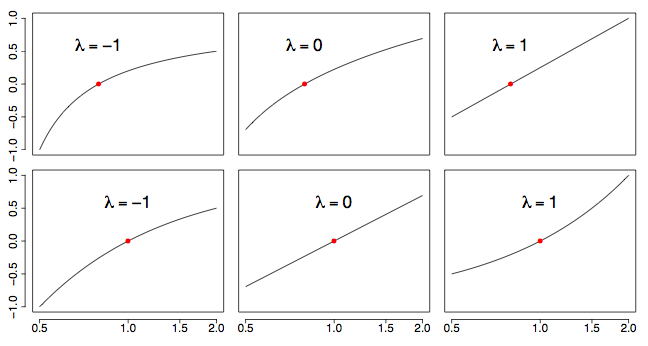
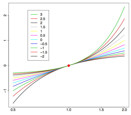
Notice with this definition of $x_{λ}^{'}$ that x = 1 always maps to the point $x_{λ}^{'}$ = 0 for all values of λ. To see how the transformation works, look at the examples in Figure 1. In the top row, the choice λ = 1 simply shifts x to the value x−1, which is a straight line. In the bottom row (on a semi-logarithmic scale), the choice λ = 0 corresponds to a logarithmic transformation, which is now a straight line. We superimpose a larger collection of transformations on a semi-logarithmic scale in Figure 2.

Six plots of the Box-Cox transformation of x for lambda = -1, 0 and 1, with a red point at (1, 0) in each. The top row plots the transformed value against x from 0.5 to 2: lambda = -1 is concave, lambda = 0 is gently concave, and lambda = 1 is exactly a straight line (x shifted to x - 1). The bottom row plots the same against log(x): now lambda = 0 is the straight line, lambda = -1 is concave and lambda = 1 is convex. — Figure 1. Examples of the Box-Cox transformation $x_{λ}^{'}$ versus x for λ = −1, 0, 1. In the second row, $x_{λ}^{'}$ is plotted against log(x). The red point is at (1, 0).

x_{λ}^{'}

x_{λ}^{'}

Family of Box-Cox transformation curves plotted against x from 0.5 to 2 on a semi-logarithmic scale, one coloured curve for each lambda from 3 down to -2 in steps of 0.5, with a legend at the upper left. Every curve passes through the red point at (1, 0); above x = 1 they fan upward in order, the lambda = 3 curve highest at about 2.3 at x = 2 and the lambda = -2 curve lowest, and the order reverses below x = 1. — Figure 2. Examples of the Box-Cox transformation $x_{λ}^{'}$ versus log(x) for −2 < λ < 3. The bottom curve corresponds to λ = −2 and the upper to λ = 3.

x_{λ}^{'}

Transformation to Normality

Another important use of variable transformation is to eliminate skewness and other distributional features that complicate analysis. Often the goal is to find a simple transformation that leads to normality. In the article on q-q plots, we discuss how to assess the normality of a set of data,

x₁,x₂,...,x_n.

Data that are normal lead to a straight line on the q-q plot. Since the correlation coefficient is maximized when a scatter diagram is linear, we can use the same approach above to find the most normal transformation.

Specifically, we form the n pairs

$(Φ^{- 1} (\frac{i - 0.5}{n}), x_{(i)}), for i = 1, 2, \dots, n$

where Φ⁻¹ is the inverse CDF of the normal density and x_(i) denotes the i^th sorted value of the data set. As an example, consider a large sample of British household incomes taken in 1973, normalized to have mean equal to one (n = 7125). Such data are often strongly skewed, as is clear from Figure 3. The data were sorted and paired with the 7125 normal quantiles. The value of λ that gave the greatest correlation (r = 0.9944) was λ = 0.21.

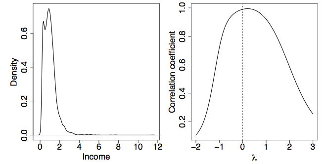
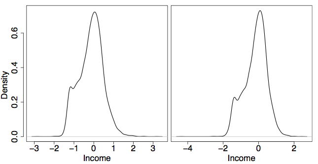
Two panels for the 1973 British household income data (n = 7125, normalised to mean 1). Left: a kernel density plot of Density against Income from 0 to 12, with a tall narrow peak of about 0.75 just below Income = 1 and a long thin right tail out past 10 — strongly positively skewed. Right: the correlation coefficient of the normal q-q pairs against lambda from -2 to 3, a smooth hump reaching almost 1.0 just to the right of the dashed line at lambda = 0; the best value is lambda = 0.21 with r = 0.9944. — Figure 3. (L) Density plot of the 1973 British income data. (R) The best value of λ is 0.21.

The kernel density plot of the optimally transformed data is shown in the left frame of Figure 4. While this figure is much less skewed than in Figure 3, there is clearly an extra "component" in the distribution that might reflect the poor. Economists often analyze the logarithm of income corresponding to λ = 0; see Figure 4. The correlation is only r = 0.9901 in this case, but for convenience, the log-transform probably will be preferred.

Two kernel density plots of the transformed 1973 British income data. Left: transformed with the optimal lambda = 0.21, on an Income axis from -3 to 3 — a near-symmetric peak of about 0.72 at 0 with a small shoulder near -1. Right: the log transform, lambda = 0, on an axis from -4 to 2 — a similar peak but with a slightly longer left tail (r = 0.9901). Both are far less skewed than the raw data, and both retain the extra low-income shoulder. — Figure 4. (L) Density plot of the 1973 British income data transformed with λ = 0.21. (R) The log-transform with λ = 0.

Other Applications

Regression analysis is another application where variable transformation is frequently applied. For the model

$y = β_{0} + β_{1} x_{1} + β_{2} x_{2} + \dots + β_{p} x_{p} + ϵ$

and fitted model

$\hat{y} = b_{0} + b_{1} x_{1} + b_{2} x_{2} + \dots + b_{p} x_{p}$

each of the predictor variables x_j can be transformed. The usual criterion is the variance of the residuals, given by

$\frac{1}{n} \sum_{i = 1}^{n} ({\hat{y}}_{i} - y_{i})^{2}$

Occasionally, the response variable y may be transformed. In this case, care must be taken because the variance of the residuals is not comparable as λ varies. Let ${\bar{g}}_{y}$ represent the geometric mean of the response variables.

${\bar{g}}_{y} = {(\prod_{i = 1}^{n} y_{i})}^{1 / n}$

Then the transformed response is defined as

$y_{λ}^{'} = \frac{y^{λ} - 1}{λ \cdot {\bar{g}}_{y}^{λ - 1}}$

When λ = 0 (the logarithmic case),

$y_{0}^{'} = {\bar{g}}_{y} \cdot \log (y)$

For more examples and discussions, see Kutner, Nachtsheim, Neter, and Li (2004).

References

Box, G. E. P. and Cox, D. R. (1964). An analysis of transformations, Journal of the Royal Statistical Society, Series B, 26, 211-252.

Kutner, M., Nachtsheim, C., Neter, J., and Li, W. (2004). Applied Linear Statistical Models, McGraw-Hill/Irwin, Homewood, IL.

Adapted from Online Statistics Education: A Multimedia Course of Study (onlinestatbook.com), Project Leader: David M. Lane, Rice University. Developed with NSF support. The original work is in the public domain; it is cited here at the authors' request. Changes were made: reformatted as an accessible XYZ web edition with native MathML. License: Public-Domain.