3.2 Measures of Spread

Variability is an important idea in statistics. If you were to measure the height of everyone in your classroom, every student gives you a different value. That means not every student has the same height. Thus, there is variability in people’s heights. If you were to take a sample of the income level of people in a town, every sample gives you different information. There is variability between samples too. Variability describes how the data are spread out. If the data are very close to each other, then there is low variability. If the data are very spread out, then there is high variability. How do you measure variability? It would be good to have a number that measures it. This section will describe some of the different measures of variability, also known as variation.

Numerical statistics for variation can show how spread out data is. The variation of data is relative, and is usually used when comparing two sets of similar data. When we are making inferences about an average, we can make better estimates when there is less variation in the data. The four most common measures of the “spread” of data are called the range, variance, standard deviation, and coefficient of variation.

A sample of house prices (in $1,000): 325, 375, 385, 395, 420, and 825, found the mean house price of $454,167. How much does this tell you about the price of all houses? Can you tell if most of the prices were close to the mean or were the prices really spread out? What is the highest price and the lowest price? All you know is that the center of the price is $454,167. What if you were approved for only $400,000 for a home loan, could you buy a home in this area? You need more information.

3.2.1 Range

The range of a set of data is the difference between the highest and the lowest data values (or maximum and minimum values). Note in statistics we only report a single number which represents the spread from the lowest to highest value.

Example 1

Look at the following three sets of data. Find the mean, median and range of each of data set.

1. 10, 20, 30, 40, 50

2. 10, 29, 30, 31, 50

3. 28, 29, 30, 31, 32

Show solution

1. Dotplot on a number line from 10 to 50 with one dot at each of 10, 20, 30, 40, and 50, showing the data spread evenly across the whole range. mean = 30, median = 30, range = 50 – 10 = 40

2. Dotplot on a number line from 10 to 50 with one dot at 10, three dots clustered at 29, 30, and 31, and one dot at 50. mean = 30, median = 30, range = 50 – 10 = 40

3. Dotplot on a number line from 10 to 50 with five dots tightly clustered from 28 to 32 and no dots elsewhere on the line. mean = 30, median = 30, range = 32 – 28 = 4

Based on the mean, median, and range, the first two distributions are the same, but you can see from the graphs that they are distributed differently. In part 1, the data are spread out equally. In part 2, the data has a clump in the middle and a single value at each end. The mean and median are the same for part 3, but the range is much smaller. All the data is clumped together in the middle.

3.2.2 Variance & Standard Deviation

The range does not really provide a very detailed picture of the variability. A better way to describe how the data is spread out is needed. Instead of looking at the distance as the highest value from the lowest, how about looking at the distance each value is from the mean? This spread is called the deviation.

Example 2

Suppose a vet wants to analyze the weights of cats. The weights (in pounds) of five cats are 6.8, 8.2, 7.5, 9.4, and 8.2. Compute the deviation for each of the data values. The deviation is how far each data point is from the mean. To be consistent always subtract the data point minus the mean.

# Cat weights (lb) -- the book's deviation -> square -> divide-by-(n-1) pipeline
w <- c(6.8, 8.2, 7.5, 9.4, 8.2)
mean(w)           # x-bar -> 8.02
sum(w - mean(w))  # deviations always sum to 0
var(w)            # s^2 = 3.728/4 -> 0.932
sd(w)             # s = sqrt(0.932) -> 0.9654

Show solution

Variable: X = weight of a cat. First, find the mean for the data set. The mean is $\bar{x}$ = $\frac{Σ (x)}{n}$ = $\frac{(6.8+8.2+7.5+9.4+8.2)}{5}$ = 8.02 pounds. Subtract the mean from each data point to get the deviations.

Figure 3-11

Now average the deviations. Add the deviations together.

Figure 3-12

The average distance from the mean cannot be zero. The reason the deviations add to 0 is that there are some positive and negative values. The sum of the deviations from the mean will always be zero.

To get rid of the negative signs square each deviation.

Figure 3-13

Then average the total of the squared deviations. The only thing is that in statistics there is a strange average here. Instead of dividing by the number of data values, you divide by the number of data values minus one. This n – 1 is called the degrees of freedom and will be discussed more later in the text. When we divide by the degrees of freedom, this gives an unbiased statistic. In this case, you would have the following:

s² = $\frac{(x - \bar{x})^{2}}{n - 1}$ = $\frac{3.728}{5 − 1}$ = $\frac{3.728}{4}$ = 0.932 pounds²

Notice that this statistic is denoted as s². This statistic is called the sample variance and it is a measure of the average squared distance from the mean. If you now take the square root, you will get the average distance from the mean. The square root of the variance is called the sample standard deviation, and is denoted with the letter s.

s= $the square root of 0.932$ = 0.9654 pounds

The standard deviation is the average (mean) distance from a data point to the mean. It can be thought of as how much a typical data point differs from the mean.

Where $\bar{x}$ is the sample mean, n is the sample size, and Σ means to find the sum.

The n – 1 in the denominator has to do with a concept called degrees of freedom (df). Dividing by the df makes the sample standard deviation a better approximation of the population standard deviation than dividing by n.

We rarely will find a population variance or standard deviation, but you will need to know the symbols.

The population variance formula: $σ^{2} = \frac{\sum (x - μ)^{2}}{N}$ .

The population standard deviation formula: $σ = \sqrt{\frac{\sum (x - μ)^{2}}{N}}$ .

The lower-case Greek letter σ pronounced “sigma” and σ² represents the population variance, μ is the population mean, and N is the size of the population.

Note: the sum of the deviations should always be zero. Try not to round too much in the calculations for standard deviation since each rounding causes a slight error.

Example 3

Suppose that a manager wants to test two new training programs. They randomly select 5 people for each training type and measures the time it takes to complete a task after the training. The times for both trainings are in table below. Which training method is more consistent?

Show solution

It is important that you define what each variable is since there are two of them.

Variable 1: X₁ = productivity from training 1

Variable 2: X₂ = productivity from training 2

The units and scale are the same for both groups. To answer which training method better, first you need some descriptive statistics. Start with the mean for each sample.

$\bar{x}$ ₁= $\frac{56 + 75 + 48 + 63 + 59}{5}$ = 60.2 minutes
$\bar{x}$ ₂= $\frac{60 + 58 + 66 + 59 + 58}{5}$ = 60.2 minutes

Since both means are the same values, you cannot answer the question about which is better.

Now calculate the standard deviation for each sample.

Figure 3-14

Figure 3-15

The variance for each sample is: \begin{aligned}
&s_{1}^{2}=\frac{394.8}{4}=98.7 \text { minutes }^{2} \\
&s_{2}^{2}=\frac{44.8}{4}=11.2 \text { minutes }^{2}
\end{aligned}

The standard deviations are: s₁= $the square root of 98.7$ = 9.9348 minutes

s₂= $the square root of 11.2$ = 3.3466 minutes.

Comparing the standard deviations, the second training method seemed to be the better training since the data is less spread out. This means it is more consistent. It would be better for the managers in this case to have a training program that produces more consistent results so they know what to expect for the time it takes to complete the task.

Descriptive statistics can be time-consuming to calculate by hand so use technology.

One Variable Statistics on the TI Calculator

The procedure for calculating the sample mean ( $\bar{x}$ ) and the sample standard deviation (s_x) for the TI calculator are shown below. Note, the TI calculator also gives you the population standard deviation (σ_x) because it does not know whether the data you input is a population or a sample. You need to decide which value you need to use, based on whether you have a population or sample. In almost all cases you have a sample and will be using s_x. In addition, the calculator uses the notation of s_x instead of just s. It is just a way for it to denote the information.

TI-84: Enter the data in a list and then press [STAT]. Use cursor keys to highlight CALC. Press 1 or [ENTER] to select 1:1-Var Stats. Press [2nd], then press the number key corresponding to your data list. Press [Enter] to calculate the statistics. Note: the calculator always defaults to L1 if you do not specify a data list.

Four TI-84 screens: data entered in list L1, the STAT CALC menu with 1:1-Var Stats highlighted, the 1-Var Stats input screen with List set to L1 and Calculate selected, and results showing x-bar = 2, Σx = 10, Σx² = 36, Sx = 2, σx = 1.788854382, and n = 5.

s_x is the sample standard deviation. You can arrow down and find more statistics. Use the min and max to calculate the range by hand. To find the variance simply square the standard deviation.

TI-89: Press [APPS], select FlashApps then press [ENTER]. Highlight Stats/List Editor then press [ENTER]. Press [ENTER] again to select the main folder. To clear a previously stored list of data values, arrow up to the list name you want to clear, press [CLEAR], then press enter.

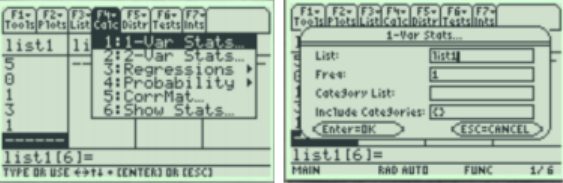
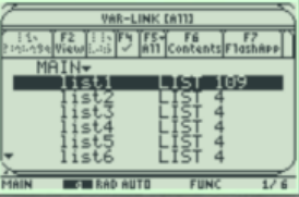
Two TI-89 Stats/List Editor screens: the F4 Calc menu with 1:1-Var Stats at the top, and the 1-Var Stats dialog with List set to list1, Freq set to 1, and Enter=OK and ESC=CANCEL buttons.

Press [F4], select 1: 1-Var Stats. To get the list name to the List box, press [2^nd] [Var-Link], arrow down to list1 and press [Enter]. This will bring list1 to the List box. Press [Enter] to enter the list name and then enter again to calculate.

Use the down arrow key to see all the statistics.

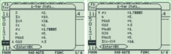
TI-89 VAR-LINK screen listing list1 through list6 in the MAIN folder, with list1 highlighted ready to be selected.

Two TI-89 1-Var Stats result screens showing x-bar = 2, Σx = 10, Σx² = 36, Sx = 2, σx = 1.78885, n = 5, MinX = 0, Q1X = 0.5, MedX = 1, Q3X = 4, MaxX = 5, and sum of squared deviations 16.

Sx is the sample standard deviation. You can arrow down and find more statistics. Use the min and max to calculate the range by hand. To find the variance simply square the standard deviation or take the last sum of squares divided by n – 1.

Excel: Type in the data into one column, select the Data tab, and choose Data Analysis. Select Descriptive Statistics, and then select OK.

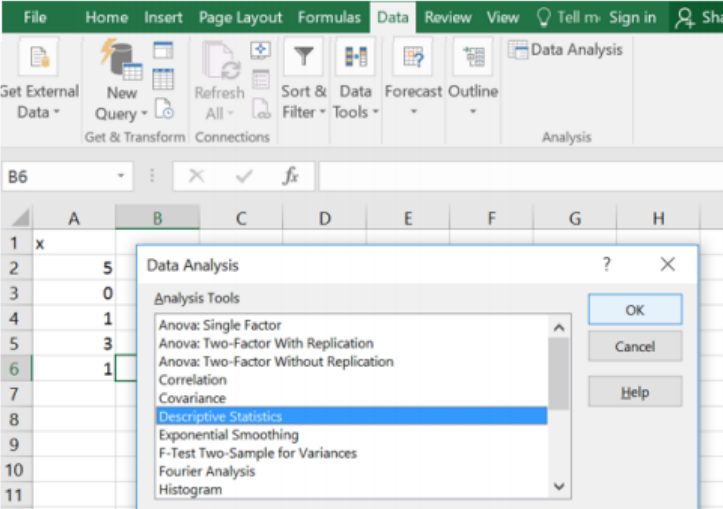
Excel Data ribbon with the Data Analysis dialog open over data values 5, 0, 1, 3, and 1 in column A; Descriptive Statistics is highlighted in the Analysis Tools list, with OK, Cancel, and Help buttons at the right.

Highlight the data for the Input Range, if you highlighted a label; check the Labels in first row box. Select the circle to the left of Output Range, then click into the box to the right of the Output Range and select one cell where you want the top left-hand corner of your summary table to start. Select the box next to Summary statistics, then select OK, see below.

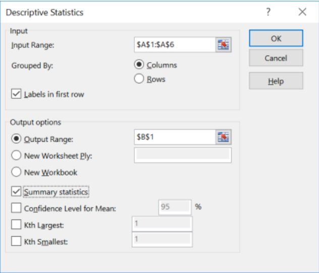
Excel Descriptive Statistics dialog with Input Range $A$1:$A$6, Grouped By set to Columns, Labels in first row checked, Output Range $B$1, and the Summary statistics box checked.

We get the following summary statistics:

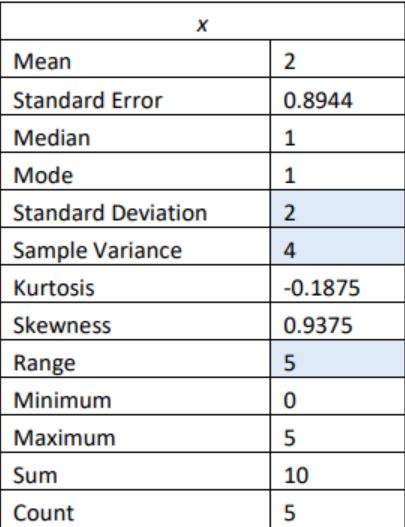
Excel summary statistics table for x: mean 2, standard error 0.8944, median 1, mode 1, standard deviation 2, sample variance 4, kurtosis −0.1875, skewness 0.9375, range 5, minimum 0, maximum 5, sum 10, and count 5.

In general, a “small” standard deviation means the data are close together (more consistent) and a “large” standard deviation means the data is spread out (less consistent). Sometimes you want consistent data and sometimes you do not. As an example, if you are making bolts, you want the lengths to be very consistent so you want a small standard deviation. If you are administering a test to see who can be a pilot, you want a large standard deviation so you can tell whom the good and bad pilots are.

What do “small” and “large” mean? To a bicyclist whose average speed is 20 mph, s = 20 mph is huge. To an airplane whose average speed is 500 mph, s = 20 mph is nothing. The “size” of the variation depends on the size of the numbers in the problem and the mean. Another situation where you can determine whether a standard deviation is small or large is when you are comparing two different samples. A sample with a smaller standard deviation is more consistent than a sample with a larger standard deviation.

If we were to compare the variability between two histograms. The standard deviation and variance measure the average spread from left to right. Take a moment and see if you can order the following histograms from the smallest to the largest standard deviation.

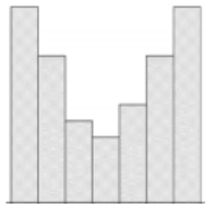
Histogram with unlabeled axes showing a U shape: the tallest bars are at the two ends and heights dip to the shortest bars in the middle.

Figure 3-16

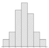
Histogram with unlabeled axes showing a bell shape: the tallest bar is at the center and bar heights step down symmetrically toward short bars at both ends.

Figure 3-17

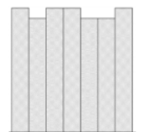
Histogram with unlabeled axes showing a roughly uniform shape: seven tall bars of nearly equal height across the whole plot.

FIgure 3-18

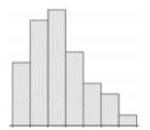
Histogram with unlabeled axes rising to a peak at the third bar and then steadily decreasing to the right, forming a mound with a longer right tail.

Figure 3-19

The histogram that has more of the data close to the mean will have the smallest standard deviation. The histogram that has more of the data towards the end points will have a larger standard deviation. Figure 3-16 will have the largest standard deviation since more of the data is grouped in the first and last class. Figure 3-17 will have the smallest standard deviation since more of the data is grouped in the center class which will be close to the mean in a symmetric distribution. Figures 3-18 and 3-19 are harder to compare without also having access to the mean and median to indicate skewness. However, Figure 3-19 does have smaller frequencies in the first and last three classes compared to Figure 3-18.

The correct order from smallest to largest standard deviation would be Figure 3-17, Figure 3-19, Figure 3-18, and then Figure 3-16.

One should not compare the range, standard deviation or variance of different data sets that have different units or scale.

3.2.3 Coefficient of Variation

The coefficient of variation, denoted by CVar or CV, is the standard deviation divided by the mean. The units on the numerator and denominator cancel with one another and the result is usually expressed as a percentage. The coefficient of variation allows you to compare variability among data sets when the units or scale is different.

Example 4

The following is a sample of the alcohol content and calories for 12 oz. beers. Is the alcohol content (alcohol by volume ABV) or calories more variable?

Name Brewery ABV Calories in 12 oz. Big Sky Scape Goat Pale Ale Big Sky Brewing 4.70% 163 Sierra Nevada Harvest Ale Sierra Nevada 6.70% 215 Steel Reserve Miller Coors 8.10% 222 O'Doul's Anheuser Busch 0.40% 70 Coors Light Miller Coors 4.15% 104 Genesee Cream Ale High Falls Brewing 5.10% 162 Breakside Pilsner Breakside 5.00% 158 Dark Ale Alberta Brewing Company 5.00% 155 Flying Dog Doggie Style Flying Dog Brewery 4.70% 158 Big Sky I.P.A. Big Sky Brewing 6.20% 195

Show solution

Type in the data to Excel and run descriptive statistics on both data sets to get the following:

Next, compute the coefficient of variation using the mean and standard deviation for both data sets.

Alcohol Content CVar = ( $\frac{0.02003}{0.05005}$ ∙ 100) % = 39.97%

Calories CVar = ( $\frac{46.39875}{160.2}$ ∙ 100) % = 28.96%

The alcohol content varies more than the number of calories.

There is no shortcut on the calculator or Excel for CVar, but you can find s and $\bar{x}$ then simply divide.

Adapted from Mostly Harmless Statistics by Rachel Webb (Portland State University), hosted on LibreTexts (stats.libretexts.org) and licensed under CC BY-SA 4.0. Changes were made. License: CC-BY-SA-4.0.