3.1 Measures of Center

Both graphical and numerical methods of summarizing data make up the branch of statistics known as descriptive statistics. Later, descriptive statistics will be used to estimate and make inferences about population parameters using methods that are part of the branch called inferential statistics. This section introduces numerical measurements to describe sample data.

This section focuses on measures of central tendency. Many times, you are asking what to expect “on average.” Such as when you pick a career, you would probably ask how much you expect to earn in that field. If you are trying to buy a home, you might ask how much homes are selling for in your area. If you are planting vegetables in your garden, you might want to know how long it will be until you can harvest. These questions, and many more, can be answered by knowing the center of the data set. The three most common measures of the “center” of the data are called the mode, mean, and median.

3.1.1 Mode

To find the mode, you count how often each data value occurs, and then determine which data value occurs most often.

There may not be a mode at all, or you may have more than one mode. If there is a tie between two values for the greatest number of times then both values are the mode and the data is called bimodal (two modes). If every data point occurs the same number of times, there is no mode. If there are more than two numbers that appear the most times, then usually we write there is no mode. When looking at grouped data in a frequency distribution or a histogram then the largest frequency is called the modal class.

Below is a dotplot showing the height of some 3-year-old children in cm and we would like to answer the question, “How tall are 3-year-olds?”

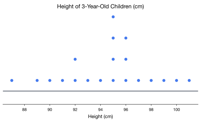
Dotplot of heights of 3-year-old children in centimeters on a number line from 87 to 101; most values have a single dot, with two dots at 92, four dots at 95, three dots at 96, and no dot at 88.

Figure 3-1

From the graph, we can see that the most frequent value is 95 cm. This is not exactly the middle of the distribution, but it is the most common height and is close to the middle in this case. We call this most frequent value the mode.

For larger data sets, use software to find the mode or at least sort the data so that you can see grouping of numbers. Excel reports a mode at the first repetitive value, so be careful in Excel with bimodal data or data with many multiples that would really have no mode at all.

Note that zero may be the most frequent value in a data set. The mode = 0 is not the same as “no mode” in the data set.

The mode is the observation that occurs most often.

Example 3-1: -5 4 8 3 4 2 0 mode = 4
Example 3-2: 3 -6 0 1 -2 1 0 5 0 mode = 0
Example 3-3: 18 25 15 32 10 27 no mode (Excel writes N/A)
Example 3-4: 15 23 18 15 24 23 17 modes = 15, 23 (bimodal)
Example 3-5: 100 125 100 125 130 140 130 140 no mode (Excel gives 100)

Summation Notation

Throughout this course, we will be using summation notation, also called sigma notation. The capital Greek letter Σ “sigma” means to add. For example, Σx means to sum up all of the x values where X is the variable name.

The order of operations is important in summation notation.

For example, Σx² = (4)² + (–3)² + (2)² + (1)² + (3)² = 39.

When we insert parentheses (Σx)² = (4 + –3 + 2 + 1 + 3)² = (7)² = 49.

Note that Σx² ≠ (Σx)².

“‘One of the interesting things about space,’ Arthur heard Slartibartfast saying to a large and voluminous creature who looked like someone losing a fight with a pink duvet and was gazing raptly at the old man's deep eyes and silver beard, ‘is how dull it is.’

‘Dull?’ said the creature, and blinked her rather wrinkled and bloodshot eyes.

‘Yes,’ said Slartibartfast, ‘staggeringly dull. Bewilderingly so. You see, there's so much of it and so little in it. Would you like me to quote some statistics?’

‘Er, well…’

‘Please, I would like to. They, too, are quite sensationally dull.’” (Adams, 2002)

3.1.2 Mean

The mean is the arithmetic average of the numbers. This is the center that most people call the average.

Distinguishing between a population and a sample is very important in statistics. We frequently use a representative sample to generalize about a population.

A statistic is any characteristic or measure from a sample. A parameter is any characteristic or measure from a population. We use sample statistics to make inferences about population parameters.

Most cases, you cannot find the population parameter, so you use the sample statistic to estimate the population parameter. Since μ cannot be calculated in most situations, the value for $\bar{x}$ is used to estimate μ. You should memorize the symbol μ and what it represents for future reference.

Example 2

Find the mean for the following sample of house prices ($1,000): 325, 375, 385, 395, 420, and 825.

Show solution

Before starting any mathematics problem, it is always a good idea to define the unknown in the problem. In this case, you want to define the variable. The symbol for the variable is x. The variable is x = price of a house in $1,000.

$\bar{x}$ = $\frac{∑x}{n}$ = $\frac{325+375+385+395+420+825}{6}$ = 454.1 $6 bar$

The sample mean house price is $454,166.67.

We can use technology to find the mean. Directions for the TI calculators are in the next section. In Excel, use the cell function AVERAGE(array). For this example, we can type the data into column A and then in a blank cell =AVERAGE(A1:A6).

3.1.3 Weighted Mean

Weighted averages are used quite often in real life. Some teachers use them in calculating your grade in the course, or your grade on a project. Some employers use them in employee evaluations. The idea is that some components of a mean are more important than others are. As an example, a full-time teacher at a community college may be evaluated on their service to the college, their service to the community, whether their paperwork is turned in on time, and their teaching. However, teaching is much more important than whether their paperwork is turned in on time. When the evaluation is completed, more weight needs to be given to the teaching and less to the paperwork. This is a weighted average.

Example 3

In your biology class, your final grade is based on several things: a lab score, scores on two major tests, and your score on the final exam. There are 100 points available for each score. The lab score is worth 15% of the course, the two exams are worth 25% of the course each, and the final exam is worth 35% of the course. Suppose you earned scores of 95 on the labs, 83 and 76 on the two exams, and 84 on the final exam. Compute your weighted average for the course.

Show solution

Variable: x = score

The weighted mean is $\frac{Σ (x w)}{Σ w}$ = $\frac{95 (0.15) + 83 (0.25) + 76 (0.25) + 84 (0.35)}{0.15 + 0.25 + 0.25 + 0.35}$ = $\frac{83.4}{1.00}$ = 83.4

The course average is 83.4 %.

Example 4

A faculty evaluation process at Portland State University rates a faculty member on the following activities: teaching, publishing, committee service, community service, and submitting paperwork in a timely manner. The process involves reviewing student evaluations, peer evaluations, and supervisor evaluation for each teacher and awarding them a score on a scale from 1 to 10 (with 10 being the best). The weights for each activity are 20 for teaching, 18 for publishing, 6 for committee service, 4 for community service, and 2 for paperwork.

a) One faculty member had the following ratings: 8 for teaching, 9 for publishing, 2 for committee work, 1 for community service, and 8 for paperwork. Compute the weighted average of their evaluation.

b) Another faculty member had ratings of 6 for teaching, 8 for publishing, 9 for committee work, 10 for community service, and 10 for paperwork. Compute the weighted average of their evaluation.

c) Which faculty member had the higher average evaluation?

Show solution

a) Variable: x = rating

The weighted average is $\frac{Σ (x w)}{\sum w}$ = $\frac{8 (20) + 9 (18) + 2 (6) + 1 (4) + 8 (2)}{20 + 18 + 6 + 4 + 2}$ = $\frac{354}{50}$ = 7.08

The average evaluation score is 7.08.

b) The weighted average is $\frac{Σ (x w)}{\sum w}$ = $\frac{6 (20) + 8 (18) + 9 (6) + 10 (4) + 10 (2)}{20 + 18 + 6 + 4 + 2}$ = $\frac{378}{50}$ = 7.56

The average evaluation score is 7.56.

c) The second faculty member has a higher average evaluation.

3.1.4 Median

Another statistic that measures the center of a distribution is the median.

To find the median:

Arrange the observations from smallest to largest.
If the number of observations n is odd, the middle observation is the median.
If the number of observations n is even, the mean of the two middle observations is the median.

We can use technology to find the median. Directions for the TI calculators are in the next section. In Excel the median is found using the cell function MEDIAN(array). For this example, we can type the data into column A and then in a blank cell =MEDIAN(A1:A6).

Recall that the sample mean house price is $454,167. Note that the median is much lower than the mean for this example. The observation of 825 is an outlier and is very large compared to the rest of the data. The sample mean is sensitive to unusual observations, i.e. outliers. The median is resistant to outliers.

3.1.5 Outliers

An outlier is a data value that is very different from the rest of the data and is far enough from the center. If there are extreme values in the data, the median is a better measure of the center than the mean. The mean is not a resistant measure because it is moved in the direction of the outlier. The median and the mode are resistant measures because they are not affected by extreme values.

As a consumer, you need to be aware that people choose the measure of center that best supports their claim. When you read an article in the newspaper and it talks about the “average,” it usually means the mean but sometimes it refers to the median. Some articles will use the word “median” instead of “average” to be more specific. If you need to make an important decision and the information says “average,” it would be wise to ask if the “average” is the mean or the median before you decide.

As an example, suppose that a company administration wants to use the mean salary as the average salary for the company. This is because the high salaries of the administration will pull the mean higher. The company can say that the employees are paid well because the average is high. However, the employees’ union wants to use the median since it discounts the extreme values of the administration and will give a lower value of the average. This will make the salaries seem lower and that a raise is in order.

Why use the mean instead of the median? When multiple samples are taken from the same population, the sample means tend to be more consistent than other measures of the center. The sample mean is the more reliable measure of center.

3.1.6 Distribution Shapes

Remember that there are varying levels of skewness and symmetry. Sample data is rarely exactly symmetric, but is approximately symmetric. Outliers will pull the mean in the direction of the outlier. If the distribution has a skewed tail to the left, the mean will be smaller than the median. If the distribution has a skewed tail to the right, the mean will be larger than the median. The mode, or modal class, is the tallest point(s), highest frequency, of the distribution. The following show examples of different distribution shapes. Figures 3-2 to 3-5 show example distribution shapes.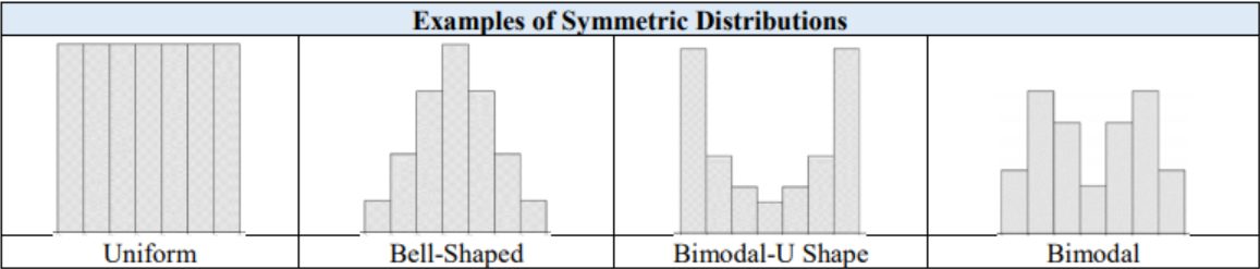 Four histograms titled Examples of Symmetric Distributions: a uniform shape with equal-height bars, a bell shape peaking at the center, a bimodal-U shape dipping in the middle with peaks at both ends, and a bimodal shape with two separate peaks.

Figure 3-2

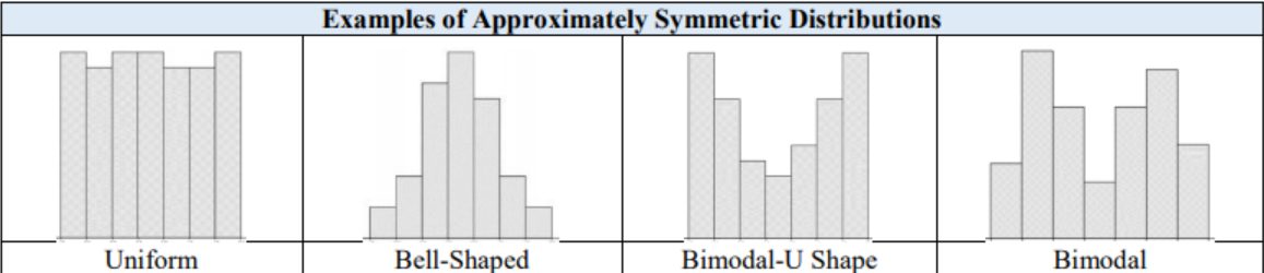
Four histograms titled Examples of Approximately Symmetric Distributions: uniform, bell-shaped, bimodal-U shape, and bimodal patterns whose bar heights are nearly, but not perfectly, mirror images left to right.

Figure 3-3

Four histograms titled Examples of Positively Skewed Distributions, each with its tallest bars toward the left and a tail of progressively shorter bars stretching to the right.

Figure 3-4

Four histograms titled Examples of Negatively Skewed Distributions, each with its tallest bars toward the right and a tail of progressively shorter bars stretching to the left. '

Figure 3-5

Comparing the mean and the median provides useful information about the distribution shape.

If the mean is equal to the median, the data is symmetric, see Figure 3-6.

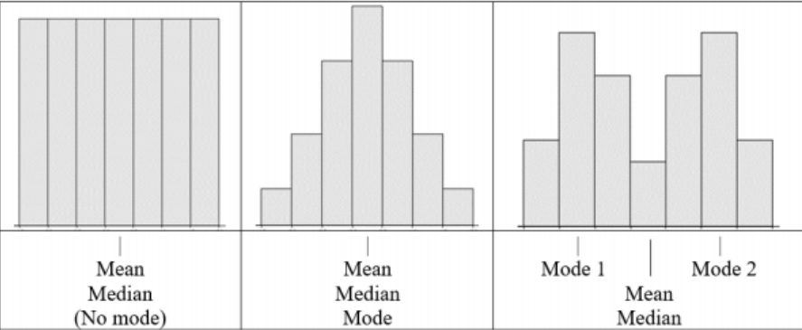
Three symmetric histograms: a uniform distribution with the mean and median marked at the center and no mode; a bell-shaped distribution with mean, median, and mode together at the center peak; and a bimodal distribution with Mode 1 and Mode 2 at its two peaks and the mean and median between them.

If the mean is larger than (to the right of) the median, the data is right skewed or positively skewed, see Figure 3-7.

If the mean is smaller than (to the left of) the median, the data is left skewed, or negatively skewed, see Figure 3-8.

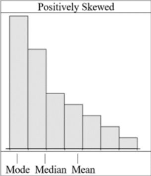
Histogram titled Positively Skewed with bars steadily decreasing in height from left to right; below the axis, the mode sits under the tallest left bar, the median is to its right, and the mean is farthest right in the tail.

Figure 3-7

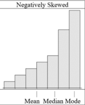
Histogram titled Negatively Skewed with bars steadily increasing in height from left to right; below the axis, the mean is farthest left in the tail, the median is in the middle, and the mode sits under the tallest right bar.

Figure 3-8

Which measure of center is used on which type of data?

Mode can be found on nominal, ordinal, interval, and ratio data, since the mode is just the data value that occurs most often. You are just counting the data values.
Median can be found on ordinal, interval, and ratio data, since you need to put the data in order. As long as there is order to the data, you can find the median.
Mean can be found on interval and ratio data, since you must have numbers to add together.

Adapted from Mostly Harmless Statistics by Rachel Webb (Portland State University), hosted on LibreTexts (stats.libretexts.org) and licensed under CC BY-SA 4.0. Changes were made. License: CC-BY-SA-4.0.