

6.3 Graphing a Line from Its Equation
Graphing a Line from Its Equation
A source-bound narrated opening with a worked example, an eight-second thinking pause, a checked result, English captions, and a transcript.
Read the transcriptDownload the videoNarration credits and licences
Recognize the Relationship Between the Solutions of an Equation and its Graph
In the previous section, we found several solutions to the equation . They are listed in Table 6.1. So, the ordered pairs , , and are some solutions to the equation . We can plot these solutions in the rectangular coordinate system as shown in Figure 6.4.
| 0 | 3 | |
| 2 | 0 | |
| 1 |
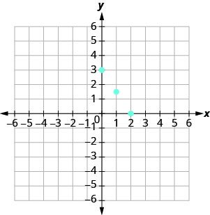
Notice how the points line up perfectly? We connect the points with a line to get the graph of the equation . See Figure 6.5. Notice the arrows on the ends of each side of the line. These arrows indicate the line continues.
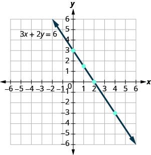
Every point on the line is a solution of the equation. Also, every solution of this equation is a point on this line. Points not on the line are not solutions.
Notice that the point whose coordinates are is on the line shown in Figure 6.6. If you substitute and into the equation, you find that it is a solution to the equation.
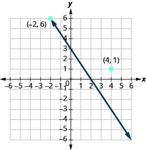
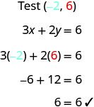
So the point is a solution to the equation . (The phrase “the point whose coordinates are ” is often shortened to “the point .”)
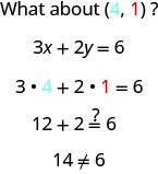
So is not a solution to the equation . Therefore, the point is not on the line. See Figure 6.5. This is an example of the saying, “A picture is worth a thousand words.” The line shows you all the solutions to the equation. Every point on the line is a solution of the equation. And, every solution of this equation is on this line. This line is called the graph of the equation .
Graph a Linear Equation by Plotting Points
There are several methods that can be used to graph a linear equation. The method we used to graph is called plotting points, or the Point–Plotting Method.
The steps to take when graphing a linear equation by plotting points are summarized below.
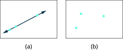
It is true that it only takes two points to determine a line, but it is a good habit to use three points. If you only plot two points and one of them is incorrect, you can still draw a line but it will not represent the solutions to the equation. It will be the wrong line.
If you use three points, and one is incorrect, the points will not line up. This tells you something is wrong and you need to check your work. Look at the difference between part (a) and part (b) in Figure 6.7.
Let’s do another example. This time, we’ll show the last two steps all on one grid.
When an equation includes a fraction as the coefficient of , we can still substitute any numbers for . But the math is easier if we make ‘good’ choices for the values of . This way we will avoid fraction answers, which are hard to graph precisely.
So far, all the equations we graphed had given in terms of . Now we’ll graph an equation with and on the same side. Let’s see what happens in the equation . If what is the value of ?
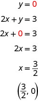
This point has a fraction for the x- coordinate and, while we could graph this point, it is hard to be precise graphing fractions. Remember in the example , we carefully chose values for so as not to graph fractions at all. If we solve the equation for , it will be easier to find three solutions to the equation.
The solutions for , , and are shown in the Table 6.4. The graph is shown in Figure 6.8.
| 0 | 3 | |
| 1 | 1 | |
| 5 |
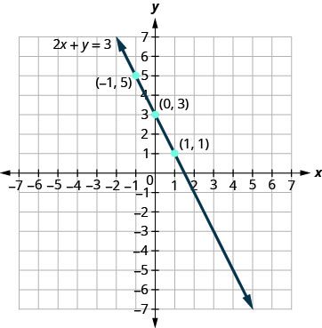
Can you locate the point , which we found by letting , on the line?
If you can choose any three points to graph a line, how will you know if your graph matches the one shown in the answers in the book? Compare two distinct points on each line. If both lines contain the same two distinct points, the graphs match. Matching x- and y-intercepts determine the same line only when the intercepts are distinct; lines through the origin can have different slopes.
The equation in Example 5 was written in standard form, with both and on the same side. We solved that equation for in just one step. But for other equations in standard form it is not that easy to solve for , so we will leave them in standard form. We can still find a first point to plot by letting and solving for . We can plot a second point by letting and then solving for . Then we will plot a third point by using some other value for or .
Practice Makes Perfect
Recognize the Relationship Between the Solutions of an Equation and its Graph
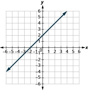
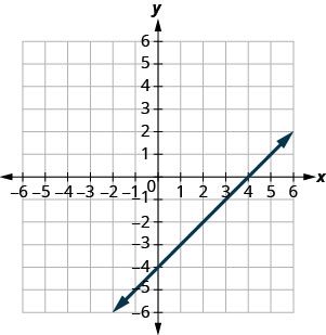
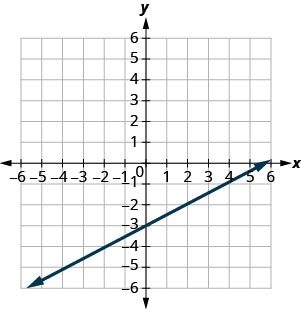
In the following exercises, for each ordered pair, decide:
ⓐ Is the ordered pair a solution to the equation? ⓑ Is the point on the line?
- ⓐ
- ⓑ
- ⓒ
- ⓓ
Show solution
ⓐ yes; yes ⓑ no; no ⓒ yes; yes ⓓ yes; yes
- ⓐ
- ⓑ
- ⓒ
- ⓓ
- ⓐ
- ⓑ
- ⓒ
- ⓓ
Show solution
ⓐ yes; yes ⓑ yes; yes ⓒ yes; yes ⓓ no; no
- ⓐ
- ⓑ
- ⓒ
- ⓓ
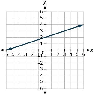
Graph a Linear Equation by Plotting Points
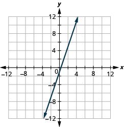
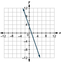
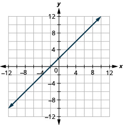
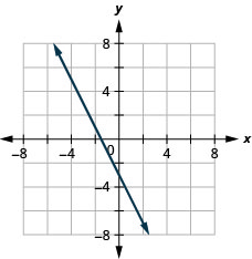
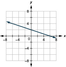
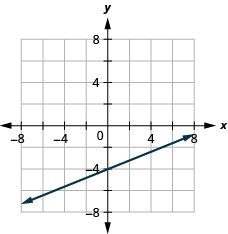
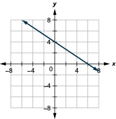
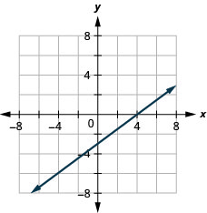
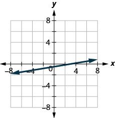
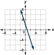
In the following exercises, graph by plotting points.
Show solution
Show solution
Show solution
Show solution
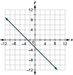
Show solution
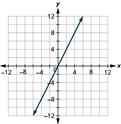
Show solution
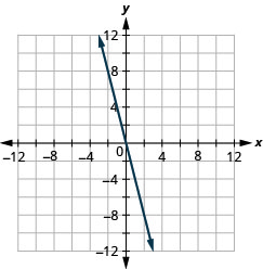
Show solution
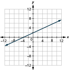
Show solution
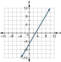
Show solution
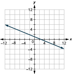
Show solution
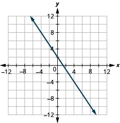
Show solution
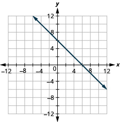
Show solution
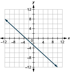
Show solution
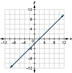
Show solution
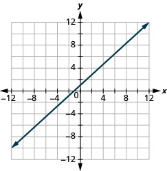
Show solution
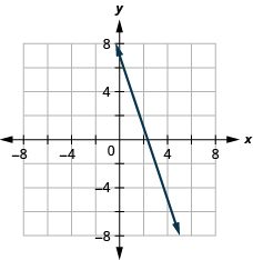
Show solution
Show solution
Show solution
Show solution
Show solution
Show solution
Show solution
Corequisite Skills for Introductory Statistics is a custom course edition compiled for Introductory Statistics corequisite courses from OpenStax Contemporary Mathematics, Elementary Algebra 2e, Intermediate Algebra 2e, Prealgebra 2e. Content by OpenStax is reproduced as published, apart from any corrections recorded for this edition. Sections are renumbered to follow the course outline. The course outline is adapted from Larry Green's Support Course for Elementary Statistics (LibreTexts, https://stats.libretexts.org/Bookshelves/Introductory_Statistics/Support_Course_for_Elementary_Statistics), used under CC BY 4.0 (https://creativecommons.org/licenses/by/4.0/). Lessons 2.4 and 6.7 are written for this edition by XYZ Homework. Every OpenStax lesson is abridged to the subsections and practice exercises this course uses. Lessons are headed with their course titles, not the source section titles. Access the complete originals free at openstax.org. License: CC-BY-NC-SA-4.0.