6.5 Solving PDEs with the Laplace Transform

The Laplace transform comes from the same family of transforms as does the Fourier seriesto the power 1, which we used in Chapter 4 to solve partial differential equations (PDEs). It is therefore not surprising that we can also solve PDEs with the Laplace transform.

Given a PDE in two independent variables $x$ and $t$ , we use the Laplace transform on one of the variables (taking the transform of everything in sight), and derivatives in that variable become multiplications by the transformed variable $s$ . The PDE becomes an ODE, which we solve. Afterwards we invert the transform to find a solution to the original problem. It is best to see the procedure on an example.

Example 1

Consider the first order PDE

$y_{t} = - α y_{x}, for x > 0, t > 0,$

with side conditions

$y (0, t) = C, y (x, 0) = 0 .$

This equation is called the convection equation or sometimes the transport equation, and it already made an appearance in Section 1.9, with different conditions. See Figure

1

for a diagram of the setup.

Figure

1

: Transport equation on a half line.

A physical setup of this equation is a river of solid goo, as we do not want anything to diffuse. The function $y$ is the concentration of some toxic substance.squared The variable $x$ denotes position where $x equals 0$ is the location of a factory spewing the toxic substance into the river. The toxic substance flows into the river so that at $x equals 0$ the concentration is always $C$ . We wish to see what happens past the factory, that is at $x greater than 0$ . Let $t$ be the time, and assume the factory started operations at $t equals 0$ , so that at $t equals 0$ the river is just pure goo.

Consider a function of two variables $y (x, t)$ . Let us fix $x$ and transform the $t$ variable. For convenience, we treat the transformed $s$ variable as a parameter, since there are no derivatives in $s$ . That is, we write $Y (x)$ for the transformed function, and treat it as a function of $x$ , leaving $s$ as a parameter.

$Y open parenthesis x close parenthesis equals L \{ y open parenthesis x, t close parenthesis \} equals ∫ 0 infinity y open parenthesis x, t close parenthesis e to the power minus s t d s.$

The transform of a derivative with respect to $x$ is just differentiating the transformed function:

$L \{ y sub x open parenthesis x, t close parenthesis \} equals ∫ 0 infinity y sub x open parenthesis x, t close parenthesis e to the power minus s t d s equals the fraction d over d x [ ∫ 0 infinity y open parenthesis x, t close parenthesis e to the power minus s t d s ] equals Y prime open parenthesis x close parenthesis.$

To transform the derivative in $t$ (the variable being transformed), we use the rules from Section 6.2:

$L \{ y sub t open parenthesis x, t close parenthesis \} equals s Y open parenthesis x close parenthesis minus y open parenthesis x, 0 close parenthesis.$

In our specific case,

y open parenthesis x, 0 close parenthesis equals 0

, and so

L \{ y sub t open parenthesis x, t close parenthesis \} equals s Y open parenthesis x close parenthesis

. We transform the equation to find

$s Y (x) = - α Y^{'} (x) .$

This ODE needs an initial condition. The initial condition is the other side condition of the PDE, the one that depends on

x

. Everything is transformed, so we must also transform this condition

$Y open parenthesis 0 close parenthesis equals L \{ y open parenthesis 0, t close parenthesis \} equals L \{ C \} equals the fraction C over s.$

We solve the ODE problem

s Y (x) = - α Y^{'} (x)

Y (0) = \frac{C}{s}

, to find

$Y (x) = \frac{C}{s} e^{- \frac{s}{α} x} .$

We are not done, we have

Y (x)

, but we really want

y (x, t)

. We transform the

s

variable back to

t

. Let

$0 if t less than 0,; 1 otherwise$

be the Heaviside function. As

$L \{ u open parenthesis t minus a close parenthesis \} equals ∫ 0 infinity u open parenthesis t minus a close parenthesis e to the power minus s t d t equals ∫ a infinity e to the power minus s t d t equals the fraction e to the power minus a s over s,$

then

$y (x, t) = L^{- 1} {\frac{C}{s} e^{- \frac{s}{α} x}} = C u (t - \frac{x}{α}) .$

In other words,

$\begin{matrix} 0 if t < \frac{x}{α}, \\ C otherwise. \end{matrix}$

See Figure $2$ for a diagram of this solution. The line of slope $\frac{1}{α}$ indicates the wavefront of the toxic substance in the picture as it is leaving the factory. What the equation does is simply move the initial condition to the right at speed $α$ .

Figure

2

: Wavefront of toxic substance is a line of slope

\frac{1}{a}

Shhh… $y$ is not differentiable, it is not even continuous (nobody ever seems to notice). How could we plug something that’s not differentiable into the equation? Well, just think of a differentiable function very very close to $y$ . Or, if you recognize the derivative of the Heaviside function as the delta function, then all is well too:

$y_{t} (x, t) = \frac{\partial}{\partial t} [C u (t - \frac{x}{α})] = C u^{'} (t - \frac{x}{α}) = C δ (t - \frac{x}{α})$

and

$y_{x} (x, t) = \frac{\partial}{\partial x} [C u (t - \frac{x}{α})] = - \frac{C}{α} u^{'} (t - \frac{x}{α}) = - \frac{C}{α} δ (t - \frac{x}{α}) .$

y_{t} = - α y_{x}

Laplace equation is very good with constant coefficient equations. One advantage of Laplace is that it easily handles nonhomogeneous side conditions. Let us try a more complicated example.

We can also detect when the problem is in the sense that it has no solution. Let us change the equation to

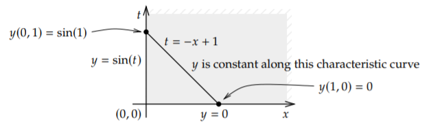
$\begin{matrix} - y_{t} + y_{x} = 0, for x > 0, t > 0, \\ y (0, t) = \sin (t), y (x, 0) = 0 . \end{matrix}$

Then the problem has no solution. First, let us see this in the language of Section 1.9. The characteristic curves are $t = - x + C$ . If $τ$ is the the characteristic coordinate, then we find the equation $y sub τ equals 0$ along the curve, meaning a solution is constant along characteristic curves. But these curves intersect both the $x$ -axis and the $t$ -axis. For example, the curve $t = - x + 1$ intersects at $open parenthesis 1, 0 close parenthesis$ and $open parenthesis 0, 1 close parenthesis$ . The solution is constant along the curve so $y open parenthesis 1, 0 close parenthesis$ should equal $y open parenthesis 0, 1 close parenthesis$ . But $y open parenthesis 1, 0 close parenthesis equals 0$ and $y (0, 1) = \sin (1) ⧸ = 0$ . See Figure $3$ .

Graph shows y is constant along t = -x+1 with y = sin(t), y(1,0) = 0 and y(0,1) = sin(1) — Figure $3$ : Ill-posed problem.

Now consider the transform. The transformed problem is

$- s Y (x) + Y^{'} (x) = 0, Y (0) = \frac{1}{s^{2} + 1},$

and the solution ought to be

$Y (x) = \frac{1}{s^{2} + 1} e^{s x} .$

Importantly, this Laplace transform does not decay to zero at infinity! That is, since

x greater than 0

in the region of interest, then

${lim}_{s \to \infty} \frac{1}{s^{2} + 1} e^{s x} = \infty ⧸ = 0 .$

It almost looks as if we could use the shifting property, but notice that the shift is in the wrong direction. Of course, we need not restrict ourselves to first order equations, although the computations become more involved for higher order equations.

Example 3

Let us use Laplace for the following problem:

$\begin{matrix} y_{t} = y_{x x}, 0 < x < \infty, t > 0, \\ y_{x} (0, t) = f (t), \\ y (x, 0) = 0 . \end{matrix}$

Really we also impose other conditions on the solution so that for example the Laplace transform exists. For example, we might impose that

y

is bounded for each fixed time

t

. Transform the equation in the

t

variable to find

$s Y (x) = Y^{″} (x) .$

The general solution to this ODE is

$Y (x) = A e^{\sqrt{s} x} + B e^{- \sqrt{s} x} .$

First

A equals 0

, since otherwise

Y

does not decay to zero as

s \to \infty

. Now consider the boundary condition. Transform

Y prime open parenthesis 0 close parenthesis equals F open parenthesis s close parenthesis

and so

- \sqrt{s} B = F (s)

. In other words,

$Y (x) = - F (s) \frac{1}{\sqrt{s}} e^{- \sqrt{s} x} .$

If we look up the inverse transform in a table such as the one in Appendix B (or we spend the afternoon doing calculus), we find

$L^{- 1} [e^{- \sqrt{s} x}] = \frac{x}{\sqrt{4 π t^{3}}} e^{\frac{- x^{2}}{4 t}},$

$L^{- 1} [\frac{1}{\sqrt{s}} e^{- \sqrt{s} x}] = \frac{1}{\sqrt{π t}} e^{\frac{- x^{2}}{4 t}} .$

$y (x, t) = L^{- 1} [F (s) e^{- \sqrt{s} x}] = \int_{0}^{t} f (τ) \frac{1}{\sqrt{π (t - τ)}} e^{\frac{- x^{2}}{4 (t - τ)}} d τ .$

Laplace can solve problems where separation of variables fails. Laplace does not mind nonhomogeneity, but it is essentially only useful for constant coefficient equations.

Footnotes

[1] There is a corresponding Fourier transform on the real line as well that looks sort of like the Laplace transform.

[2] It’s a river of goo already, we’re not hurting the environment much more.

Adapted from Differential Equations for Engineers by Jiří Lebl (Oklahoma State University), hosted on LibreTexts (math.libretexts.org) and licensed under CC BY-SA 4.0. Changes were made. License: CC-BY-SA-4.0.