6.2 Transforms of derivatives and ODEs

Transforms of derivatives

Let us see how the Laplace transform is used for differential equations. First let us try to find the Laplace transform of a function that is a derivative. Suppose $g (t)$ is a differentiable function of exponential order, that is, $| g open parenthesis t close parenthesis | less than or equal to M e to the power c t$ for some $M$ and $c$ . So $ℒ { g open parenthesis t close parenthesis }$ exists, and what is more, ${lim}_{t \to \infty} e^{- s t} g (t) = 0$ when $s > c$ . Then

$ℒ {g^{'} (t)} = \int_{0}^{\infty} e^{- s t} g^{'} (t) d t = {[e^{- s t} g (t)]}_{t = 0}^{\infty} - \int_{0}^{\infty} (- s) e^{- s t} g (t) d t = - g (0) + s ℒ {g (t)} .$

We repeat this procedure for higher derivatives. The results are listed in Table $1$ . The procedure also works for piecewise smooth functions, that is functions that are piecewise continuous with a piecewise continuous derivative. The fact that the function is of exponential order is used to show that the limits appearing above exist. We will not worry much about this fact.

Table $1$ : Laplace transforms of derivatives ( $G open parenthesis s close parenthesis equals ℒ { g open parenthesis t close parenthesis }$ as usual).
$f (t)$	$ℒ { f open parenthesis t close parenthesis } equals F open parenthesis s close parenthesis$
$g^{'} (t)$	$s G open parenthesis s close parenthesis minus g open parenthesis 0 close parenthesis$
$g^{″} (t)$	$s^{2} G (s) - s g (0) - g^{'} (0)$
$g^{‴} (t)$	$s^{3} G (s) - s^{2} g (0) - s g^{'} (0) - g^{″} (0)$

Solving ODEs with the Laplace Transform

Notice that the Laplace transform turns differentiation into multiplication by $s$ . Let us see how to apply this fact to differential equations.

Example 1

Take the equation

$x^{″} (t) + x (t) = \cos (2 t), x (0) = 0, x^{'} (0) = 1 .$

We will take the Laplace transform of both sides. By $X (s)$ we will, as usual, denote the Laplace transform of $x (t)$ .

$\begin{matrix} ℒ {x^{″} (t) + x (t)} = ℒ {\cos (2 t)}, \\ s^{2} X (x) - s x (0) + x^{'} (0) + X (s) = \frac{s}{s^{2} + 4} . \end{matrix}$

We plug in the initial conditions now—this makes the computations more streamlined—to obtain

$s^{2} X (s) - 1 + X (s) = \frac{s}{s^{2} + 4} .$

We solve for $X (s)$ ,

$X (s) = \frac{s}{(s^{2} + 1) (s^{2} + 4)} + \frac{1}{s^{2} + 1} .$

We use partial fractions (exercise) to write

$X (s) = \frac{1}{3} \frac{s}{s^{2} + 1} - \frac{1}{3} \frac{s}{s^{2} + 4} + \frac{1}{s^{2} + 1} .$

Now take the inverse Laplace transform to obtain

$x (t) = \frac{1}{3} \cos (t) - \frac{1}{3} \cos (2 t) + \sin (t) .$

The procedure for linear constant coefficient equations is as follows. We take an ordinary differential equation in the time variable $t$ . We apply the Laplace transform to transform the equation into an algebraic (non differential) equation in the frequency domain. All the $x (t)$ , $x^{'} (t)$ , $x^{″} (t)$ , and so on, will be converted to $X (s)$ , $s X open parenthesis s close parenthesis minus x open parenthesis 0 close parenthesis$ , $s^{2} X (s) - s x (0) - x^{'} (0)$ , and so on. We solve the equation for $X (s)$ . Then taking the inverse transform, if possible, we find $x (t)$ .

It should be noted that since not every function has a Laplace transform, not every equation can be solved in this manner. Also if the equation is not a linear constant coefficient ODE, then by applying the Laplace transform we may not obtain an algebraic equation.

Using the Heaviside Function

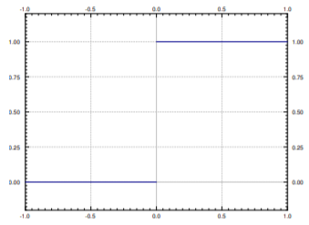
Before we move on to more general equations than those we could solve before, we want to consider the Heaviside function. See Figure $1$ for the graph.

$0 i f t less than 0,; 1 i f t greater than or equal to 0.$

Graph that includes the negative x-axis and the horizontal right directional ray starting at (0,1) — Figure $1$ : Plot of the Heaviside (unit step) function $u (t)$ .

This function is useful for putting together functions, or cutting functions off. Most commonly it is used as $u (t - a)$ for some constant $a$ . This just shifts the graph to the right by $a$ . That is, it is a function that is 0 when $< a$ and 1 when $t \geq a$ . Suppose for example that $f (t)$ is a “signal” and you started receiving the signal $\sin t$ at time $t = π$ . The function $f (t)$ should then be defined as

$0 i f t less than π,; sin t i f t greater than or equal to π.$

Using the Heaviside function, $f (t)$ can be written as

$f (t) = u (t - π) \sin t$

Similarly the step function that is $1$ on the interval $[ 1, 2 close parenthesis$ and zero everywhere else can be written as

$u (t - 1) - u (t - 2) .$

The Heaviside function is useful to define functions defined piecewise. If you want to define $f (t)$ such that $f (t) = t$ when $t$ is in $[ 0, 1 ]$ , $f (t) = - t + 2$ when $t$ is in $[ 1, 2 close parenthesis$ and $f open parenthesis t close parenthesis equals 0$ otherwise, you can use the expression

$f (t) = t (u (t) - u (t - 1)) + (- t + 2) (u (t - 1) - u (t - 2)) .$

Hence it is useful to know how the Heaviside function interacts with the Laplace transform. We have already seen that

$ℒ {u (t - a)} = \frac{e^{- a s}}{2} .$

Shifting Property

This can be generalized into a shifting property or second shifting property.

$ℒ {f (t - a) u (t - a)} = e^{- a s} ℒ {f (t)} .$

(6.2.1)

Example 2

Suppose that the forcing function is not periodic. For example, suppose that we had a mass-spring system

$x^{″} (t) + x (t) = f (t), x (0) = 0, x^{'} (0) = 0,$

where $f open parenthesis t close parenthesis equals 1$ if $1 less than or equal to t less than 5$ and zero otherwise. We could imagine a mass-spring system, where a rocket is fired for 4 seconds starting at $t equals 1$ . Or perhaps an RLC circuit, where the voltage is raised at a constant rate for 4 seconds starting at $t equals 1$ , and then held steady again starting at $t equals 5$ .

We can write $f (t) = u (t - 1) - u (t - 5)$ . We transform the equation and we plug in the initial conditions as before to obtain

$s^{2} X (s) + X (s) = \frac{e^{- s}}{s} - \frac{e^{- 5 s}}{s} .$

We solve for $X (s)$ to obtain

$X (s) = \frac{e^{- s}}{s (s^{2} + 1)} - \frac{e^{- 5 s}}{s (s^{2} + 1)} .$

We leave it as an exercise to the reader to show that

$ℒ^{- 1} {\frac{1}{s (s^{2} + 1)}} = 1 - \cos t .$

In other words $ℒ {1 - \cos t} = \frac{1}{s (s^{2} + 1)}$ . So using (6.2.1) we find

$ℒ^{- 1} {\frac{e^{- s}}{s (s^{2} + 1)}} = ℒ^{- 1} {e^{- s} ℒ {1 - \cos t}} = (1 - \cos (t - 1)) u (t - 1) .$

Similarly

$ℒ^{- 1} {\frac{e^{- 5 s}}{s (s^{2} + 1)}} = ℒ^{- 1} {e^{- 5 s} ℒ {1 - \cos t}} = (1 - \cos (t - 5)) u (t - 5) .$

Hence, the solution is

$x (t) = (1 - \cos (t - 1)) u (t - 1) - (1 - \cos (t - 5)) u (t - 5) .$

The plot of this solution is given in Figure $2$ .

The section's own solution of x″ + x = f(t), x(0) = x′(0) = 0, namely x(t) = (1 − cos(t−1))u(t−1) − (1 − cos(t−1−d))u(t−1−d), with time t on the horizontal axis and the burn now lasting d seconds — the book's case is d = 4, a rocket fired for 4 seconds starting at t = 1. Drag d to π (≈ 3.14) for the loudest possible aftermath, amplitude exactly 2; then on to 2π (≈ 6.28), where the two cosine pieces cancel and the mass returns to rest and stays there. The leftover ringing is 2|sin(d/2)|, so it depends only on the burn length modulo the natural period 2π — not on how long ago the burn ended.

Figure

2

: Plot of

x (t)

Transfer Functions

Laplace transform leads to the following useful concept for studying the steady state behavior of a linear system. Suppose we have an equation of the form

$L x = f (t),$

where $L$ is a linear constant coefficient differential operator. Then $f (t)$ is usually thought of as input of the system and $x (t)$ is thought of as the output of the system. For example, for a mass-spring system the input is the forcing function and output is the behavior of the mass. We would like to have an convenient way to study the behavior of the system for different inputs.

Let us suppose that all the initial conditions are zero and take the Laplace transform of the equation, we obtain the equation

$A (s) X (s) = F (s) .$

Solving for the ratio $\frac{X (s)}{F (s)}$ we obtain the so-called transfer function $H (s) = \frac{1}{A (s)}$ .

$H (s) = \frac{X (s)}{F (s)}$

In other words, $X (s) = H (s) F (s)$ . We obtain an algebraic dependence of the output of the system based on the input. We can now easily study the steady state behavior of the system given different inputs by simply multiplying by the transfer function.

Example 3

Given $x^{″} + ω_{0}^{2} x = f (t)$ , let us find the transfer function (assuming the initial conditions are zero).

First, we take the Laplace transform of the equation.

$s^{2} X (s) + ω_{0}^{2} X (s) = F (s) .$

Now we solve for the transfer function $\frac{X (s)}{F (s)}$ .

$H (s) = \frac{X (s)}{F (s)} = \frac{1}{s^{2} + ω_{0}^{2}} .$

Let us see how to use the transfer function. Suppose we have the constant input $f open parenthesis t close parenthesis equals 1$ . Hence $F (s) = \frac{1}{s}$ , and

$X (s) = H (s) F (s) = \frac{1}{s^{2} + ω_{0}^{2}} \frac{1}{s} .$

Taking the inverse Laplace transform of $X (s)$ we obtain

$x (t) = \frac{1 - \cos (ω_{0} t)}{ω_{0}^{2}} .$

Transforms of Integrals

A feature of Laplace transforms is that it is also able to easily deal with integral equations. That is, equations in which integrals rather than derivatives of functions appear. The basic property, which can be proved by applying the definition and doing integration by parts, is

$ℒ {\int_{0}^{t} f (τ) d τ} = \frac{1}{s} F (s) .$

It is sometimes useful (e.g. for computing the inverse transform) to write this as

$\int_{0}^{t} f (τ) d τ = ℒ^{- 1} {\frac{1}{s} F (s)} .$

Example 4

To compute $ℒ^{- 1} {\frac{1}{s (s^{2} + 1)}}$ we could proceed by applying this integration rule.

$ℒ^{- 1} {\frac{1}{2} \frac{1}{s^{2} + 1}} = \int_{0}^{t} ℒ^{- 1} {\frac{1}{s^{2} + 1}} = \int_{0}^{t} \sin τ d τ = 1 - \cos t .$

Example 5

An equation containing an integral of the unknown function is called an integral equation. For example, take

$t^{2} = \int_{0}^{t} e^{τ} x (τ) d τ$

where we wish to solve for $x (t)$ . We apply the Laplace transform and the shifting property to get

$\frac{2}{s^{3}} = \frac{1}{s} ℒ {e^{t} x (t)} = \frac{1}{s} X (s - 1),$

where $X open parenthesis s close parenthesis equals ℒ { x open parenthesis t close parenthesis }$ . Thus

$X (s - 1) = \frac{2}{s^{2}} or X (s) = \frac{2}{(s + 1)^{2}} .$

We use the shifting property again to get

$x (t) = 2 e^{- t} t .$

Adapted from Differential Equations for Engineers by Jiří Lebl (Oklahoma State University), hosted on LibreTexts (math.libretexts.org) and licensed under CC BY-SA 4.0. Changes were made. License: CC-BY-SA-4.0.