6.1 The Laplace Transform

Transform

In this chapter we will discuss the Laplace transformto the power 1. The Laplace transform turns out to be a very efficient method to solve certain ODE problems. In particular, the transform can take a differential equation and turn it into an algebraic equation. If the algebraic equation can be solved, applying the inverse transform gives us our desired solution. The Laplace transform also has applications in the analysis of electrical circuits, NMR spectroscopy, signal processing, and elsewhere. Finally, understanding the Laplace transform will also help with understanding the related Fourier transform, which, however, requires more understanding of complex numbers.

The Laplace transform also gives a lot of insight into the nature of the equations we are dealing with. It can be seen as converting between the time and the frequency domain. For example, take the standard equation

$m x^{″} (t) = c x^{'} (t) + k x (t) = f (t) .$

We can think of $t$ as time and $f (t)$ as incoming signal. The Laplace transform will convert the equation from a differential equation in time to an algebraic (no derivatives) equation, where the new independent variable $s$ is the frequency.

We can think of the Laplace transform as a black box that eats functions and spits out functions in a new variable. We write $ℒ { f open parenthesis t close parenthesis } equals F open parenthesis s close parenthesis$ for the Laplace transform of $f (t)$ . It is common to write lower case letters for functions in the time domain and upper case letters for functions in the frequency domain. We use the same letter to denote that one function is the Laplace transform of the other. For example $F (s)$ is the Laplace transform of $f (t)$ . Let us define the transform.

$ℒ {f (t)} = F (s) \overset{d e f}{=} \int_{0}^{\infty} e^{- s t} f (t) d t .$

We note that we are only considering $t greater than or equal to 0$ in the transform. Of course, if we think of $t$ as time there is no problem, we are generally interested in finding out what will happen in the future (Laplace transform is one place where it is safe to ignore the past). Let us compute some simple transforms.

Example 1

Suppose $f open parenthesis t close parenthesis equals 1$ , then

$ℒ {1} = \int_{0}^{\infty} e^{- s t} d t = {[\frac{e^{- s t}}{- s}]}_{t = 0}^{\infty} = {lim}_{h \to \infty} {[\frac{e^{- s t}}{- s}]}_{t = 0}^{h} = {lim}_{h \to \infty} (\frac{e^{- s h}}{- s} - \frac{1}{- s}) = \frac{1}{s} .$

The limit (the improper integral) only exists if $s greater than 0$ . So $ℒ { 1 }$ is only defined for $s greater than 0$ .

Example 2

Suppose $f (t) = e^{- a t}$ , then

$ℒ {e^{- a t}} = \int_{0}^{\infty} e^{- s t} e^{- a t} d t = \int_{0}^{\infty} e^{- (s + a) t} d t = {[\frac{e^{- (s + a) t}}{- s (s + a)}]}_{t = 0}^{\infty} = \frac{1}{s + a} .$

The limit only exists if $s plus a greater than 0$ . So $ℒ {e^{- a t}}$ is only defined for $s plus a greater than 0$ .

Example 3

Suppose $f (t) = t$ , then using integration by parts

$\begin{matrix} ℒ {t} = \int_{0}^{\infty} e^{- s t} t d t \\ = {[\frac{- t e^{- s t}}{s}]}_{t = 0}^{\infty} + \frac{1}{s} \int_{0}^{\infty} e^{- s t} d t \\ = 0 + \frac{1}{s} {[\frac{e^{- s t}}{- s}]}_{t = 0}^{\infty} \\ = \frac{1}{s^{2}} . \end{matrix}$

Again, the limit only exists if $s greater than 0$ .

Example 4

A common function is the unit step function, which is sometimes called the Heaviside functionsquared. This function is generally given as

$0 i f t less than 0,; 1 i f t greater than or equal to 0.$

Let us find the Laplace transform of $u (t - a)$ , where $a greater than or equal to 0$ is some constant. That is, the function that is 0 for $t < a$ and 1 for $t \geq a$ .

$ℒ {u (t - a)} = \int_{0}^{\infty} e^{- s t} u (t - a) d t = \int_{a}^{\infty} e^{- s t} d t = {[\frac{e^{- s t}}{- s}]}_{t = a}^{e^{- a s}} = \frac{e^{- a s}}{s},$

where of course $s greater than 0$ (and $a greater than or equal to 0$ as we said before).

By applying similar procedures we can compute the transforms of many elementary functions. Many basic transforms are listed in Table $1$ .

Table $1$ : Some Laplace transforms ( $C, ω$ , and $a$ are constants).
$f (t)$	${ f open parenthesis t close parenthesis }$
$C$	$\frac{C}{s}$
$t$	$\frac{1}{s^{2}}$
$t^{2}$	$\frac{2}{s^{3}}$
$t^{3}$	$\frac{6}{s^{4}}$
$t^{n}$	$\frac{n!}{s^{s + 1}}$
$e^{- a t}$	$\frac{1}{s + a}$
$\sin (ω t)$	$\frac{ω}{s^{2} + ω^{2}}$
$\cos (ω t)$	$\frac{s}{s^{2} + ω^{2}}$
$\sinh (ω t)$	$\frac{ω}{s^{2} - ω^{2}}$
$\cosh (ω t)$	$\frac{s}{s^{2} - ω^{2}}$
$u (t - a)$	$\frac{e^{- a s}}{s}$

Since the transform is defined by an integral. We can use the linearity properties of the integral. For example, suppose $C$ is a constant, then

$ℒ {f (t)} = \int_{o}^{\infty} e^{- s t} C f (t) d t = C \int_{0}^{\infty} e^{- s t} f (t) d t = C ℒ {f (t)} .$

So we can “pull out” a constant out of the transform. Similarly we have linearity. Since linearity is very important we state it as a theorem.

Note

Linearity of the Laplace Transform

Suppose that $A$ , $B$ , and $C$ are constants, then

$ℒ {A f (t) + B g (t)} = A ℒ {f (t)} + B ℒ {g (t)}$

and in particular

$ℒ { C f open parenthesis t close parenthesis } equals C ℒ { f open parenthesis t close parenthesis }.$

These rules together with Table $1$ make it easy to find the Laplace transform of a whole lot of functions already. But be careful. It is a common mistake to think that the Laplace transform of a product is the product of the transforms. In general

$ℒ { f open parenthesis t close parenthesis g open parenthesis t close parenthesis } not equal to ℒ { f open parenthesis t close parenthesis } ℒ { g open parenthesis t close parenthesis }.$

It must also be noted that not all functions have a Laplace transform. For example, the function $1 / t$ does not have a Laplace transform as the integral diverges for all $s$ . Similarly, $\tan t$ or $e^{t^{2}}$ do not have Laplace transforms.

Existence and Uniqueness

Let us consider when does the Laplace transform exist in more detail. First let us consider functions of exponential order. The function $f (t)$ is of exponential order as $t$ goes to infinity if

$| f open parenthesis t close parenthesis | less than or equal to M e to the power c t,$

for some constants $M$ and $c$ , for sufficiently large $t$ (say for all $t > t_{o}$ for some $t_{o}$ ). The simplest way to check this condition is to try and compute

${lim}_{t \to \infty} \frac{f (t)}{e^{c t}}$

If the limit exists and is finite (usually zero), then $f (t)$ is of exponential order.

For an exponential order function we have existence and uniqueness of the Laplace transform.

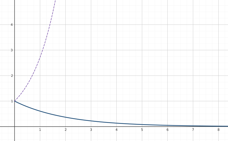
Function graph showing y = exp((1-s)*t) on t in [0, 20] and y = exp(t) on t in [0, 20]. Adjustable parameter: Transform variable s (s) = 1.5. Viewing window: x from -0.57 to 8.37, y from -0.56 to 4.96. — The existence theorem's own integral, drawn. For f(t) = e^t — of exponential order with c = 1 — the transform integrand e^(−st) f(t) = e^((1−s)t) is the solid curve, with f itself dashed behind it, and only t ≥ 0 is plotted because the definition integrates from 0 to ∞. Drag s down through the threshold s = c = 1: above it the integrand decays and the improper integral converges, so F(s) exists; at s = 1 it flattens to the constant 1 and the area is already infinite; below it the integrand grows and there is no transform at all.

The existence is not difficult to see. Let $f (t)$ be of exponential order, that is $| f open parenthesis t close parenthesis | less than or equal to M e to the power c t$ for all $t greater than 0$ (for simplicity $t sub 0 equals 0$ ). Let $s > c$ , or in other words $open parenthesis c minus s close parenthesis less than 0$ . By the comparison theorem from calculus, the improper integral defining $ℒ { f open parenthesis t close parenthesis }$ exists if the following integral exists

$\int_{0}^{\infty} e^{- s t} (M e^{c t}) d t = M \int_{0}^{\infty} e^{(c - s) t} d t = M {[\frac{e^{(c - s) t}}{c - s}]}_{t = 0}^{\infty} = \frac{M}{c - s} .$

The transform also exists for some other functions that are not of exponential order, but that will not be relevant to us. Before dealing with uniqueness, let us note that for exponential order functions we obtain that their Laplace transform decays at infinity:

$lim sub s → infinity F open parenthesis s close parenthesis equals 0$

Both theorems hold for piecewise continuous functions as well. Recall that piecewise continuous means that the function is continuous except perhaps at a discrete set of points where it has jump discontinuities like the Heaviside function. Uniqueness however does not “see” values at the discontinuities. So we can only conclude that $F (s) = G (s)$ outside of discontinuities. For example, the unit step function is sometimes defined using $u open parenthesis 0 close parenthesis equals 1 / 2$ . This new step function, however, has the exact same Laplace transform as the one we defined earlier where $u open parenthesis 0 close parenthesis equals 1$ .

6.1.3Inverse Transform

As we said, the Laplace transform will allow us to convert a differential equation into an algebraic equation. Once we solve the algebraic equation in the frequency domain we will want to get back to the time domain, as that is what we are interested in. If we have a function $F (s)$ , to be able to find $f (t)$ such that $ℒ { f open parenthesis t close parenthesis } equals F open parenthesis s close parenthesis$ , we need to first know if such a function is unique. It turns out we are in luck by Theorem $3$ . So we can without fear make the following definition.

If $F open parenthesis s close parenthesis equals ℒ { f open parenthesis t close parenthesis }$ for some function $f (t)$ . We define the inverse Laplace transform as

$ℒ^{- 1} {F (s)} \overset{d e f}{=} f (t)$

There is an integral formula for the inverse, but it is not as simple as the transform itself—it requires complex numbers and path integrals. For us it will suffice to compute the inverse using Table $1$ .

Example 5

Find the inverse Laplace transform of $F (s) = \frac{1}{s + 1}$

Show solution

We look at the table to find

$ℒ^{- 1} {\frac{1}{s + 1}} = e^{- t}$

As the Laplace transform is linear, the inverse Laplace transform is also linear. That is,

$ℒ^{- 1} {A F (s) + B G (s)} = A ℒ^{- 1} {F (s)} + B ℒ^{- 1} {G (s)}$

Of course, we also have $ℒ^{- 1} {A F (s) = A ℒ^{- 1} {F (s)} .$ Let us demonstrate how linearity can be used.

Example 6

Find the inverse Laplace transform of

$F (s) = \frac{s^{2} + s + 1}{s^{3} + s} .$

Show solution

First we use the method of partial fractions to write $F$ in a form where we can use Table $1$ . We factor the denominator as $s open parenthesis s squared plus 1 close parenthesis$ and write

$\frac{s^{2} + s + 1}{s^{3} + s} = \frac{A}{s} + \frac{B s + C}{s^{2} + 1}$

Putting the right hand side over a common denominator and equating the numerators we get $A (s^{2} + 1) + s (B s + C) = s^{2} + s + 1$ . Expanding and equating coefficients we obtain $A + B = 1$ , $C equals 1$ , $A equals 1$ and thus $B equals 0$ . In other words,

$F (s) = \frac{s^{2} + s + 1}{s^{3} + s} = \frac{1}{s} + \frac{1}{s^{2} + 1}$

By linearity of the inverse Laplace transform we get

$ℒ^{- 1} {\frac{s^{2} + s + 1}{s^{3} + s}} = ℒ^{- 1} {\frac{1}{s}} + ℒ^{- 1} {\frac{1}{s^{2} + 1}} = 1 + \sin t .$

Shifting Property of Laplace Transforms

Another useful property is the so-called shifting property or the first shifting property

$ℒ {e^{- a t} f (t)} = F (s + a)$

where $F (s)$ is the Laplace transform of $f (t)$ and $a$ is a constant.

The shifting property can be used, for example, when the denominator is a more complicated quadratic that may come up in the method of partial fractions. We complete the square and write such quadratics as $(s + a)^{2} + b$ and then use the shifting property.

Example 7

Find

$ℒ^{- 1} {\frac{1}{s^{2} + 4 s + 8}} .$

Show solution

First we complete the square to make the denominator $(s + 2)^{2} + 4$ . Next we find

$ℒ {\frac{1}{s^{2} + 4}} = \frac{1}{2} \sin (2 t) .$

Putting it all together with the shifting property, we find

$ℒ {\frac{1}{s^{2} + 4 s + 8}} = ℒ {\frac{1}{(s + 2)^{2} + 4}} = \frac{1}{2} e^{- 2 t} \sin (2 t) .$

In general, we want to be able to apply the Laplace transform to rational functions, that is functions of the form

$\frac{F (s)}{G (s)}$

where $F (s)$ and $G (s)$ are polynomials. Since normally, for the functions that we are considering, the Laplace transform goes to zero as $s \to \infty$ , it is not hard to see that the degree of $F (s)$ must be smaller than that of $G (s)$ . Such rational functions are called proper rational functions and we can always apply the method of partial fractions. Of course this means we need to be able to factor the denominator into linear and quadratic terms, which involves finding the roots of the denominator,

Footnotes

[1] Just like the Laplace equation and the Laplacian, the Laplace transform is also named after Pierre-Simon, marquis de Laplace (1749 – 1827).

[2] The function is named after the English mathematician, engineer, and physicist Oliver Heaviside (1850–1925). Only by coincidence is the function “heavy” on “one side.”

Adapted from Differential Equations for Engineers by Jiří Lebl (Oklahoma State University), hosted on LibreTexts (math.libretexts.org) and licensed under CC BY-SA 4.0. Changes were made. License: CC-BY-SA-4.0.