We said that the Laplace transformation of a product is not the product of the transforms. All hope is not lost however. We simply have to use a different type of a “product.” Take two functions and defined for , and define the convolution1 of and as
(6.3.1)
As you can see, the convolution of two functions of is another function of .
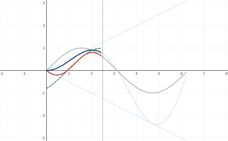
Interactive figureConvolution as flip-and-slide, and where resonance comes fromDrag the t and Frequency ω sliders.
XYZ Graph · viewer build 5edf91b
Lebl's Example 6.3.2 worked as a picture: (sin ωt ∗ cos ωt)(t) = ½ t sin(ωt). The pale curve is f(τ) = sin(ωτ), fixed. The dashed curve is g(t − τ) = cos(ω(t − τ)) — g REVERSED and slid to the right by t, which is the whole content of the definition ∫₀ᵗ f(τ)g(t − τ)dτ. The heavy orange curve is their product, drawn only on 0 ≤ τ ≤ t, and its signed area is the answer. Drag t: the window widens, the reversed copy slides, and the bold blue curve is TRACED OUT as you go — that is the running result, and the pale blue curve ahead of it is where it is headed. Notice the blue curve does not just oscillate — it grows inside the dashed ±t/2 envelope. That factor of t is why §2.6's resonance solution grows without bound, and here you can watch it accumulate rather than take it from the algebra.
The convolution has many properties that make it behave like a product. Let be a constant and , , and be functions then
The most interesting property for us, and the main result of this section is the following theorem.
In other words, the Laplace transform of a convolution is the product of the Laplace transforms. The simplest way to use this result is in reverse.
Solving ODEs
The next example demonstrates the full power of the convolution and the Laplace transform. We can give the solution to the forced oscillation problem for any forcing function as a definite integral.
Volterra Integral Equation
A common integral equation is the Volterra integral equation2
where and are known functions and is an unknown we wish to solve for. To find , we apply the Laplace transform to the equation to obtain
where , , and are the Laplace transforms of , , and , respectively. We find
To find we now need to find the inverse Laplace transform of .
Footnotes
[1] For those that have seen convolution defined before, you may have seen it defined as . This definition agrees with (6.3.1) if you define and to be zero for . When discussing the Laplace transform the definition we gave is sufficient. Convolution does occur in many other applications, however, where you may have to use the more general definition with infinities.
[2] Named for the Italian mathematician Vito Volterra (1860–1940).
These eBooks are a prerelease and are not yet certified conformant with WCAG 2.1 AA or ADA Title II. Every page is built against an automated accessibility gate, and the published editions will meet ADA Title II requirements when they release in late September 2026. If something is unusable, please tell us.