Often in applications we study a physical system by putting in a short pulse and then seeing what the system does. The resulting behavior is often called impulse response. Let us see what we mean by a pulse. The simplest kind of a pulse is a simple rectangular pulse defined by
Notice that
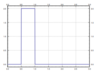
where is the unit step function (see Figure for a graph).
Figure : Sample square pulse with , , and .
Let us take the Laplace transform of a square pulse,
For simplicity we let and it is convenient to set to have
That is, to have the pulse have “unit mass.” For such a pulse we compute
We generally want to be very small. That is, we wish to have the pulse be very short and very tall. By letting go to zero we arrive at the concept of the Dirac delta function.
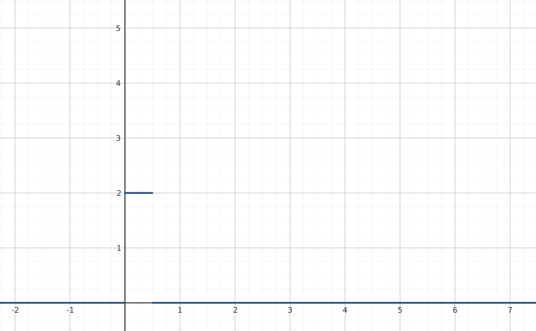
Interactive figureUnit-mass pulse φ(t) as b → 0Drag the Pulse width b slider from 0.2 to 4.
XYZ Graph · viewer build 5edf91b
The book's own normalized pulse φ(t) = (u(t) − u(t−b))/b — the a = 0, M = 1/b case this section sets up right before it takes the limit — with time t on the horizontal axis. Drag b from 4 down to 0.2 and watch the rectangle go short-and-wide → tall-and-thin: the height 1/b is not chosen, it is forced by the area staying exactly 1, which is precisely the limit that defines δ(t). At b = 0.5 the rectangle is 0.5 wide and 2 tall — the same shape as the book's own sample square pulse (a = 0.5, b = 1, M = 2), slid back to start at the origin. There are no vertical sides at t = 0 and t = b: those are genuine jump discontinuities, not gaps in the drawing.
6.4.2Delta Function
The Dirac delta function1 is not exactly a function; it is sometimes called a generalized function. We avoid unnecessary details and simply say that it is an object that does not really make sense unless we integrate it. The motivation is that we would like a “function” such that for any continuous function we have
The formula should hold if we integrate over any interval that contains 0, not just . So is a “function” with all its “mass” at the single point . In other words, for any interval
Unfortunately there is no such function in the classical sense. You could informally think that is zero for and somehow infinite at .
A good way to think about is as a limit of short pulses whose integral is 1. For example, suppose that we have a square pulse as above with , , that is .
Compute
If is continuous at , then for very small , the function is approximately equal to on the interval . We approximate the integral
Therefore,
Let us therefore accept as an object that is possible to integrate. We often want to shift to another point, for example . In that case we have
Note that is the same object as . In other words, the convolution of with is again ,
As we can integrate , let us compute its Laplace transform.
In particular,
Impulse Response
As we said before, in the differential equation , we think of as input, and as the output. Often it is important to find the response to an impulse, and then we use the delta function in place of . The solution to
is called the impulse response.
Let us notice something about the above example. In Example 6.3.4, we found that when the input was , then the solution to was given by
Notice that the solution for an arbitrary input is given as convolution with the impulse response. Let us see why. The key is to notice that for functions and ,
We simply differentiate twice under the integral,2 the details are left as an exercise. And so if we convolve the entire equation (6.4.1), the left hand side becomes
The right hand side becomes
Therefore is the solution to
This procedure works in general for other linear equations . If you determine the impulse response, you also know how to obtain the output for any input by simply convolving the impulse response and the input .
Three-Point Beam Bending
Let us give another quite different example where the delta function turns up: Representing point loads on a steel beam. Consider a beam of length , resting on two simple supports at the ends. Let denote the position on the beam, and let denote the deflection of the beam in the vertical direction. The deflection satisfies the Euler-Bernoulli equation,3
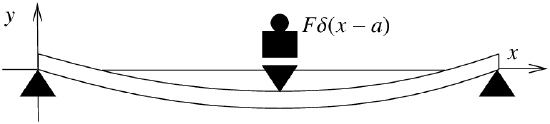
where and are constants4 and is the force applied per unit length at position . The situation we are interested in is when the force is applied at a single point as in Figure .
Figure : Three-point bending.
In this case the equation becomes
where is the point where the mass is applied. is the force applied and the minus sign indicates that the force is downward, that is, in the negative direction. The end points of the beam satisfy the conditions,
See Section 5.2, for further information about endpoint conditions applied to beams.
Footnotes
[1] Named after the English physicist and mathematician Paul Adrien Maurice Dirac (1902–1984).
[2] You should really think of the integral going over rather than over and simply assume that and are continuous and zero for negative.
[3] Named for the Swiss mathematicians Jacob Bernoulli (1654–1705), Daniel Bernoulli —nephew of Jacob— (1700–1782), and Leonhard Paul Euler (1707–1783).
[4] is the elastic modulus and is the second moment of area. Let us not worry about the details and simply think of these as some given constants.
These eBooks are a prerelease and are not yet certified conformant with WCAG 2.1 AA or ADA Title II. Every page is built against an automated accessibility gate, and the published editions will meet ADA Title II requirements when they release in late September 2026. If something is unusable, please tell us.