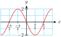
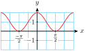
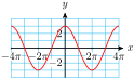
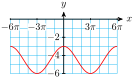
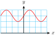
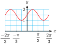
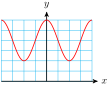
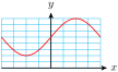
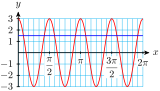
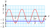
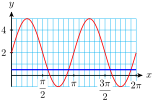
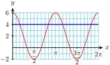
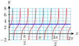
In Chapter 4 we saw that the amplitude, period, and midline of a sinusoidal graph are determined by the coefficients in its formula. The circular functions (sine and cosine of real numbers) behave the same way.
Period, Midline, and Amplitude
Changes to the amplitude, period, and midline are called transformations of the basic sine and cosine graphs.
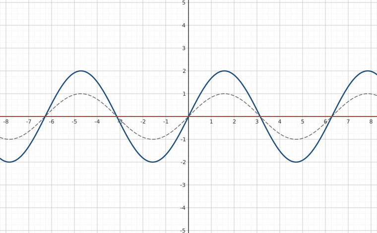
Interactive figureAmplitude and midline of y = a sin x + kDrag the Amplitude a and Midline k sliders.
XYZ Graph · viewer build 5edf91b
The transformations this section studies, applied live to y = a sin x + k against the basic graph y = sin x (gray). The slider a stretches the wave vertically: the amplitude is |a|, and dragging a negative reflects the graph about its midline — compare a = 2 with a = −2. The slider k slides the whole wave up or down: the dashed line y = k is the midline, and the graph always stays within |a| of it. Neither slider changes where the wave crosses its midline — the period stays 2π — which is exactly why amplitude, midline, and period are three independent transformations.
Changing the midline shifts the graph vertically.
Changing the amplitude stretches or compresses the graph vertically.
Changing the period stretches or compresses the graph horizontally.
First, we'll consider changes in amplitude.
The amplitude of is given by , and the same is true of . In the next exercise, remember that the amplitude is always a nonnegative number.
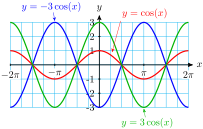
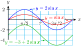
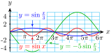
Compare the graphs of and with the graph of .
Both graphs have amplitude 3. The graph of is reflected about the -axis.
Next, we'll consider changes in the period of the graph.
The period of is given by , and the same is true of .
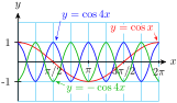
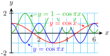
Compare the graph of with the graph of for .
Compare the graph of with the graph of for .
The graph of completes 3 cycles from to . Its period is .
The graph of completes one cycle from to . Its period is .
Next we'll consider changes in midline.
Compare the graph of with the graph of .
The graph of is shifted down 3 units. Its midline is .
Here is a summary of our findings.
Graphs of Sinusoidal Functions
The values of the parameters determine the shape of the graphs of
By adjusting the amplitude, period, and midline of the sine or cosine graph, we can sketch these sinusoidal functions.
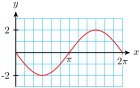
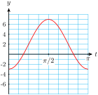
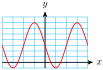
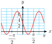
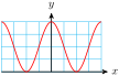
State the amplitude, period, and midline of the graph of .
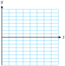
Complete the table and sketch a graph of .
Amplitude: 2, period: , midline: .
Modeling with Sinusoidal Functions
Sinusoidal functions are used to model a great variety of physical phenomena, including sound and light waves, tides and planetary orbits, and the life cycles of plants and animals. They are also often used to approximate periodic functions that are not exactly sinusoidal, such as blood pressure.
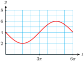
In the next Checkpoint, note the starting point of the graph, and choose the most appropriate sinusoidal function to model the function.
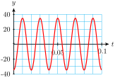
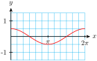
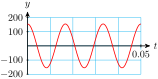
The graph below shows the voltage of a generator, as seen on an oscilloscope.
Write a sinusoidal function for the voltage level.
What is the frequency of the signal, in cycles per second?
50 cycles per second
The Tangent Function
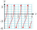
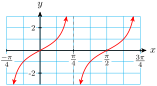
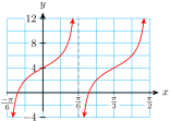
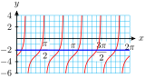
The transformations of shifting and stretching can be applied to the tangent function as well. The graph of does not have an amplitude, but we can see any vertical stretch by comparing the function values at the guidepoints.
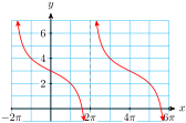
Identify the midline and period of the tangent graph shown below.
Find an equation of the form
for the graph.
Midline: , period
Review the following skills you will need for this section.
Section 7.1 Summary
Vocabulary
Transformation
Amplitude
Period
Midline
Concepts
Changes to the amplitude, period, and midline of the basic sine and cosine graphs are called transformations. Changing the midline shifts the graph vertically, changing the amplitude stretches or compresses the graph vertically, and changing the period stretches or compresses the graph horizontally.
One way to make a quick sketch of a sinusoidal graph is to use a table of values. The trick is to choose convenient values for the input variable.
The transformations of shifting and stretching can be applied to the tangent function as well.
Study Questions
Count from to by multiples of .
Count from to by multiples of .
Transformationhe maximum value of a certain sinusoidal function is , and its minimum value is . What is the midline of the function? What is its amplitude?
, and . What are the values of and ?
Skills
Identify the amplitude, period, and midline of a circular function #1–8, 23–30
Graph a circular function #9–16, 31–44
Find a formula for the graph of a circular function #17–30
Model periodic phenomena with circular functions #45–52
Graph transformations of the tangent function #535–8
Solve trigonometric equations graphically #59–70
Homework 7-1
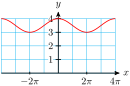
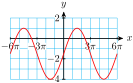
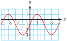
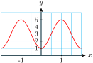
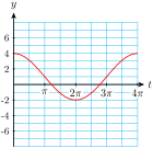
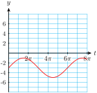
For Problems 1–8, state the amplitude, period, and midline of the graph.
amplitude , period , midline
amplitude , period , midline
amplitude , period , midline
amplitude , period , midline
In Problems 9–16, we use transformations to sketch graphs of the functions in Problems 1–8. Sketch one cycle of each graph by hand and label scales on the axes.
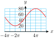
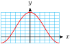
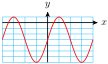
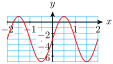
For Problems 17–22, write an equation for the graph using sine or cosine.
For Problems 23–30,
State the amplitude, period, and midline of the graph.
Write an equation for the graph using sine or cosine.
amplitude , period , midline
amplitude , period , midline
amplitude , period , midline
amplitude , period , midline
In Problems 31–36, we use a table of values to sketch circular functions.
Complete the table of values for the function.
Sketch a graph of the function and label the scales on the axes.
For Problems 37–44, label the scales on the axes for the graph.
The height of the tide in Cabot Cove can be approximated by a sinusoidal function. At 5 am on July 23, the water level reached its high mark at the 20-foot line on the pier, and at 11 am, the water level was at its lowest at the 4-foot line.
Sketch a graph of , the water level as a function of time, from 5 am on July 23 to 5 am on July 24.
Write an equation for the function.
The population of mosquitoes at Marsh Lake is a sinusoidal function of time. The population peaks around June 1 at about 6000 mosquitoes per square kilometer, and is smallest on December 1, at 1000 mosquitoes per square kilometer.
Sketch a graph of , the number of mosquitoes as a function of the month, where on June 1.
Write an equation for the function.
The paddlewheel on the Delta Queen steamboat is 28 feet in diameter, and is rotating once every ten seconds. The bottom of the paddlewheel is 4 feet below the surface of the water.
The ship's logo is painted on one of the paddlewheel blades. At , the blade with the logo is at the top of the wheel. Sketch a graph of the logo's heightabove the water as a function of .
Write an equation for the function.
Delbert's bicycle wheel is 24 inches in diameter, and he has a light attached to the spokes 10 inches from the center of the wheel. It is dark, and he is cycling home slowly from work. The bicycle wheel makes one revolution every second.
At , the light is at its highest point the bicycle wheel. Sketch a graph of the light's height as a function of .
Write an equation for the function.
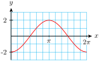
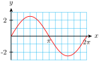
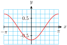
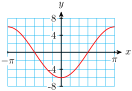
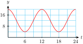
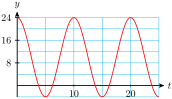
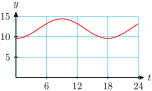
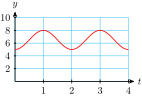
For Problems 49–52, write an equation for the sinusoidal function whose graph is shown.
The number of hours of daylight in Salt Lake City varies from a minimum of 9.6 hours on the winter solstice to a maximum of 14.4 hours on the summer solstice. Time is measured in months, starting at the winter solstice.
A weight is 6.5 feet above the floor, suspended from the ceiling by a spring. The weight is pulled down to 5 feet above the floor and released, rising past 6.5 feet in 0.5 second before attaining its maximum height of 8 feet. The weight oscillates between its minimum and maximum height.
The voltage used in U.S. electrical current changes from 155V to 155V and back 60 times each second.
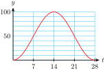
Although the moon is spherical, what we see from earth looks like a disk, sometimes only partly visible. The percentage of the moon's disk that is visible varies between 0 (at new moon) to 100 (at full moon), over a 28-day cycle.
For Problems 53–58,
Make a table of values and sketch a graph of the function.
Give its period and midline.
undef
undef
period , midline
undef
undef
period , midline
undef
undef
period , midline
For Problems 59–64, use the graph to find all solutions between and .
, , , , , , ,
, , ,
, , , , ,
For Problems 65–70,
Use technology to graph the function for .
Use the intersect feature to find all solutions between and . Round your answers to hundredths.
Trigonometry by Katherine Yoshiwara (yoshiwarabooks.org), GNU Free Documentation License 1.2 or later. Adapted for the XYZ HTML edition with the authors' permission (recorded 2026-07-04). License: GFDL-1.2-or-later.
These eBooks are a prerelease and are not yet certified conformant with WCAG 2.1 AA or ADA Title II. Every page is built against an automated accessibility gate, and the published editions will meet ADA Title II requirements when they release in late September 2026. If something is unusable, please tell us.