14.5 Parametric Equations

As we have seen in Exercises - in Section 5.5, Chapter 8 and most recently in Section 14.2, there are scores of interesting curves which, when plotted in the $x y$ -plane, neither represent $y$ as a function of $x$ nor $x$ as a function of $y$ .

In this section, we present a new concept which allows us to use functions to study these kinds of curves. To motivate the idea, we imagine a bug crawling across a table top starting at the point $O$ and tracing out a curve $C$ in the plane, as shown below.

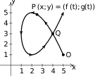
Coordinate-plane figure. — **Figure 14.207**

The curve $C$ does not represent $y$ as a function of $x$ because it fails the Vertical Line Test and it does not represent $x$ as a function of $y$ because it fails the Horizontal Line Test.

However, since the bug can be in only one place $P (x, y)$ at any given time $t$ , we can define the $x$ -coordinate of $P$ as a function of $t$ and the $y$ -coordinate of $P$ as a (usually, but not necessarily) different function of $t$ . Traditionally, $f (t)$ is used for $x$ and $g (t)$ is used for $y$ .

The independent variable $t$ in this case is called a parameter and the system of equations

${\begin{matrix} x & = & f (t) \\ y & = & g (t) \end{matrix}$

is called a system of parametric equations or a parametrization of the curve $C$ .¹

The parametrization of $C$ endows it with an orientation and the arrows on $C$ indicate motion in the direction of increasing values of $t$ .

In this case, our bug starts at the point $O$ , travels upwards to the left, then loops back around to cross its path² at the point $Q$ and finally heads off into the first quadrant.

It is important to note that the curve itself is a set of points and as such is devoid of any orientation. The parametrization determines the orientation and as we shall see, different parametrizations can determine different orientations.

If all of this seems hauntingly familiar, it should. By definition, the system of equations ${x = \cos (t), y = \sin (t)$ parametrizes the Unit Circle, giving it a counter-clockwise orientation.

More generally, the equations of circular motion ${x = r \cos (ω t), y = r \sin (ω t)$ developed on page 11.3 in Section 11.2.1 are parametric equations which trace out a circle of radius $r$ centered at the origin.

If $ω greater than 0$ , the orientation is counter-clockwise; if $ω less than 0$ , the orientation is clockwise. The angular frequency $ω$ determines `how fast' the object moves around the circle.

In particular, the equations ${x = 2960 \cos (\frac{π}{12} t), y = 2960 \sin (\frac{π}{12} t)$ that model the motion of Lakeland Community College as the earth rotates (see Example 11.2.6 in Section 11.2.1) parameterize a circle of radius 2960 with a counter-clockwise rotation which completes one revolution as $t$ runs through the interval $open bracket 0, 24 close parenthesis$ . It is time for another example.

Example 1

Sketch the curve described by ${\begin{matrix} x & = & t^{2} - 3 \\ y & = & 2 t - 1 \end{matrix}$ for $t greater than or equal to minus 2.$

We follow the same procedure here as we have time and time again when asked to graph anything new – choose values for $t$ , then plot and connect the corresponding points.

Since we are told $t greater than or equal to minus 2$ , we start there and as we plot successive points, we draw an arrow to indicate the direction of the path for increasing values of $t$ .

$\begin{matrix} t & x (t) & y (t) & (x (t), y (t)) \\ - 2 & 1 & - 5 & (1, - 5) \\ - 1 & - 2 & - 3 & (- 2, - 3) \\ 0 & - 3 & - 1 & (- 3, - 1) \\ 1 & - 2 & 1 & (- 2, 1) \\ 2 & 1 & 3 & (1, 3) \\ 3 & 6 & 5 & (6, 5) \end{matrix}$

Figure 14.208

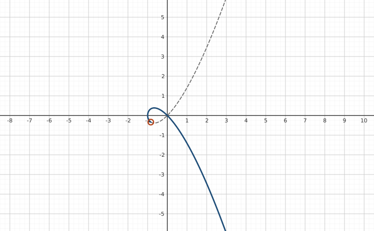
The curve sketched out in Example 14.5.1 certainly looks like a parabola, and the presence of the $t^{2}$ term in the equation $x = t^{2} - 3$ reinforces this hunch.

Since the parametric equations ${x = t^{2} - 3, y = 2 t - 1$ given to describe this curve are a system of equations, we can use the technique of substitution as described in Section 9.7 to eliminate the parameter $t$ and get an equation involving just $x$ and $y$ .

To do so, we choose to solve the equation $y = 2 t - 1$ for $t$ to get $t = \frac{y + 1}{2}$ . Substituting this into the equation $x = t^{2} - 3$ yields $x = {(\frac{y + 1}{2})}^{2} - 3$ or, after some rearrangement, ${(y + 1)}^{2} = 4 (x + 3)$ .

Thinking back to Section 8.2, we see that the graph of this equation is a parabola with vertex $(- 3, - 1)$ which opens to the right, as required.

Technically speaking, the equation ${(y + 1)}^{2} = 4 (x + 3)$ describes the entire parabola, while the parametric equations ${x = t^{2} - 3, y = 2 t - 1$ for $t greater than or equal to minus 2$ describe only a portion of the parabola.

In this case,³ we can remedy this situation by restricting the bounds on $y$ . Since the portion of the parabola we want is exactly the part where $y greater than or equal to minus 5$ , the equation ${(y + 1)}^{2} = 4 (x + 3)$ coupled with the restriction $y greater than or equal to minus 5$ describes the same curve as the given parametric equations. The one piece of information we can never recover after eliminating the parameter, however, is the orientation of the curve.

Eliminating the parameter and obtaining an equation in terms of $x$ and $y$ , whenever possible, can be a great help in graphing curves determined by parametric equations.

If the system of parametric equations contains algebraic functions, as was the case in Example 14.5.1, then the usual techniques of substitution and elimination as learned in Section 9.7 can be applied to the system ${x = f (t), y = g (t)$ to eliminate the parameter.

If, on the other hand, the parametrization involves the trigonometric functions, the strategy changes slightly. In this case, it is often best to solve for the trigonometric functions and relate them using an identity.

We demonstrate these techniques in the following example.

Example 2

Sketch the curves described by the following parametric equations.

${\begin{matrix} x & = & t^{3} \\ y & = & 2 t^{2} \end{matrix}$ for $minus 1 less than or equal to t less than or equal to 1$
${\begin{matrix} x & = & e^{- t} \\ y & = & e^{- 2 t} \end{matrix}$ for $t greater than or equal to 0$
${\begin{matrix} x & = & \sin (t) \\ y & = & \csc (t) \end{matrix}$ for $0 less than t less than π$
${\begin{matrix} x & = & 1 + 3 \cos (t) \\ y & = & 2 \sin (t) \end{matrix}$ for $0 \leq t \leq \frac{3 π}{2}$

To get a feel for the curve described by the system ${x = t^{3}, y = 2 t^{2}$ we first sketch the graphs of $x = t^{3}$ and $y equals 2 ⁢ t squared$ over the interval $open bracket minus 1, 1 close bracket$ below on the left in the middle, respectively.
We note that as $t$ takes on values in the interval $open bracket minus 1, 1 close bracket$ , $x = t^{3}$ ranges between $minus 1$ and $1$ , and $y equals 2 ⁢ t squared$ ranges between $0$ and $2$ . This means that all of the action is happening on a portion of the plane, namely $open brace open parenthesis x, y close parenthesis vertical bar minus 1 less than or equal to x less than or equal to 1, 0 less than or equal to y less than or equal to 2 close brace$ .
Next, we plot a few points to get a sense of the position and orientation of the curve. Certainly, $t = - 1$ and $t equals 1$ are good values to pick since these are the extreme values of $t$ . We also choose $t equals 0$ , since that corresponds to a (local) minimum⁴ on the graph of $y equals 2 ⁢ t squared$ . Plugging in $t = - 1$ gives the point $open parenthesis minus 1, 2 close parenthesis$ , $t equals 0$ gives $open parenthesis 0, 0 close parenthesis$ and $t equals 1$ gives $open parenthesis 1, 2 close parenthesis$ .
More generally, we see that $x = t^{3}$ is increasing over the entire interval $open bracket minus 1, 1 close bracket$ whereas $y equals 2 ⁢ t squared$ is decreasing over the interval $open bracket minus 1, 0 close bracket$ and then increasing over $open bracket 0, 1 close bracket$ .
Geometrically, this means that in order to trace out the path described by the parametric equations, we start at $open parenthesis minus 1, 2 close parenthesis$ (where $t = - 1$ ), then move to the right (since $x$ is increasing) and down (since $y$ is decreasing) to $open parenthesis 0, 0 close parenthesis$ (where $t equals 0$ ).
We continue to move to the right (since $x$ is still increasing) but now move upwards (since $y$ is now increasing) until we reach $open parenthesis 1, 2 close parenthesis$ (where $t equals 1$ ).
Finally, to get a good sense of the shape of the curve, we eliminate the parameter. Solving $x = t^{3}$ for $t$ , we get $t = \sqrt[3]{x}$ . Substituting this into $y equals 2 ⁢ t squared$ gives $y = 2 {(\sqrt[3]{x})}^{2} = 2 x^{2 / 3}$ . Our experience in Section 4.2 yields the graph of our final answer below on the right.
Figure 14.209
Figure 14.210
Figure 14.211
$x = t^{3}$ , $minus 1 less than or equal to t less than or equal to 1$
$y equals 2 ⁢ t squared$ , $minus 1 less than or equal to t less than or equal to 1$
${x = t^{3}, y = 2 t^{2}$ , $minus 1 less than or equal to t less than or equal to 1$
For the system ${x = 2 e^{- t}, y = e^{- 2 t}$ for $t greater than or equal to 0$ , we proceed as in the previous example and graph $x = 2 e^{- t}$ and $y = e^{- 2 t}$ over the interval $open bracket 0, ∞ close parenthesis$ below on the left and in the middle, respectively.
We find that the range of $x$ in this case is $open parenthesis 0, 2 close bracket$ and the range of $y$ is $open parenthesis 0, 1 close bracket$ , so our graph will reside in a portion of Quadrant I: $open brace open parenthesis x, y close parenthesis vertical bar 0 less than x less than or equal to 2, 0 less than y less than or equal to 1 close brace$ .
Next, we plug in some friendly values of $t$ to get a sense of the orientation of the curve. Since $t$ lies in the exponent here, `friendly' values of $t$ involve natural logarithms. Starting with $t = \ln (1) = 0$ we get⁵ $open parenthesis 2, 1 close parenthesis$ , for $t equals ln ⁡ open parenthesis 2 close parenthesis$ we get $(1, \frac{1}{4})$ and for $t equals ln ⁡ open parenthesis 3 close parenthesis$ we get $(\frac{2}{3}, \frac{1}{9})$ .
Since $t$ is ranging over the unbounded interval $open bracket 0, ∞ close parenthesis$ , we take the time to analyze the end behavior of both $x$ and $y$ . We find $lim_{t \to \infty} x (t) = lim_{t \to \infty} 2 e^{- t} = 0$ and $lim_{t \to \infty} y (t) = lim_{t \to \infty} e^{- 2 t} = 0$ This means the graph of ${x = 2 e^{- t}, y = e^{- 2 t}$ approaches the point $open parenthesis 0, 0 close parenthesis$ .
Since both $x = 2 e^{- t}$ and $y = e^{- 2 t}$ are always decreasing for $t greater than or equal to 0$ , we know that our final graph will start at $open parenthesis 2, 1 close parenthesis$ (where $t equals 0$ ), and move consistently to the left (since $x$ is decreasing) and down (since $y$ is decreasing) to approach the origin.
To eliminate the parameter, one way to proceed is to solve $x = 2 e^{- t}$ for $t$ to get $t = - \ln (\frac{x}{2})$ . Substituting this for $t$ in $y = e^{- 2 t}$ gives $y = e^{- 2 (- \ln (x / 2))} = e^{2 \ln (x / 2)} = e^{\ln {(x / 2)}^{2}} = {(\frac{x}{2})}^{2} = \frac{x^{2}}{4}$ .
Alternatively, we could recognize that $y = e^{- 2 t} = {(e^{- t})}^{2}$ , and since $x = 2 e^{- t}$ means $e^{- t} = \frac{x}{2}$ , we get $y = {(\frac{x}{2})}^{2} = \frac{x^{2}}{4}$ this way as well.
Either way, the graph of ${x = 2 e^{- t}, y = e^{- 2 t}$ for $t greater than or equal to 0$ is a portion of the parabola $y = \frac{x^{2}}{4}$ which starts at the point $open parenthesis 2, 1 close parenthesis$ and heads towards, but never reaches,⁶ $open parenthesis 0, 0 close parenthesis$ as seen below on the right.
Figure 14.212
Figure 14.213
Figure 14.214
$x = 2 e^{- t}$ , $t greater than or equal to 0$
$y = e^{- 2 t}$ , $t greater than or equal to 0$
${x = 2 e^{- t}, y = e^{- 2 t}$ , $t greater than or equal to 0$
For the system ${x = \sin (t), y = \csc (t)$ for $0 less than t less than π$ , we start by graphing $x = \sin (t)$ and $y = \csc (t)$ over the interval $open parenthesis 0, π close parenthesis$ below on the left and in the middle, respectively.
We find that the range of $x$ is $open parenthesis 0, 1 close bracket$ while the range of $y$ is $open bracket 1, ∞ close parenthesis$ which means our graph will lie in the first quadrant.
Plotting a few friendly points, we see that $t = \frac{π}{6}$ gives the point $(\frac{1}{2}, 2)$ , $t = \frac{π}{2}$ gives $open parenthesis 1, 1 close parenthesis$ and $t = \frac{5 π}{6}$ returns us to $(\frac{1}{2}, 2)$ .
Since $t equals 0$ and $t = π$ aren't included in the domain for $t$ , (because $y = \csc (t)$ is undefined at these $t$ -values), we analyze the behavior of the system as $t$ approaches $0$ and $π$ .
We have $lim_{t \to 0^{+}} x (t) = lim_{t \to 0^{+}} \sin (t) = 0$ and $lim_{t \to π^{-}} x (t) = lim_{t \to π^{-}} \sin (t) = 0$ . Also, $lim_{t \to 0^{+}} y (t) = lim_{t \to 0^{+}} \csc (t) = \infty$ and $lim_{t \to π^{-}} y (t) = lim_{t \to π^{-}} \csc (t) = \infty$ . Piecing all of this information together, we get that for $t$ near $0$ , we have points with very small positive $x$ -values, but very large positive $y$ -values.
As $t$ ranges through the interval $(0, \frac{π}{2}]$ , $x = \sin (t)$ is increasing and $y = \csc (t)$ is decreasing. This means that we are moving to the right and downwards, through $(\frac{1}{2}, 2)$ when $t = \frac{π}{6}$ to $open parenthesis 1, 1 close parenthesis$ when $t = \frac{π}{2}$ . Once $t = \frac{π}{2}$ , the orientation reverses, and we start to head to the left, since $x = \sin (t)$ is now decreasing, and up, since $y = \csc (t)$ is now increasing. We pass back through $(\frac{1}{2}, 2)$ when $t = \frac{5 π}{6}$ back to the points with small positive $x$ -coordinates and large positive $y$ -coordinates.
Figure 14.215
Figure 14.216
Figure 14.217
$x = \sin (t)$ , $0 less than t less than π$
$y = \csc (t)$ , $0 less than t less than π$
${x = \sin (t), y = \csc (t)$ , $0 less than t less than π$
To better explain this behavior, we eliminate the parameter. Using a reciprocal identity, we write $y = \csc (t) = \frac{1}{\sin (t)}$ . Since $x = \sin (t)$ , the curve traced out by this parametrization is a portion of the graph of $y = \frac{1}{x}$ . We now can explain the unusual behavior as $t \to 0^{+}$ and $t \to π^{-}$ – for these values of $t$ , we are hugging the vertical asymptote $x equals 0$ of the graph of $y = \frac{1}{x}$ .
We see that the parametrization given above traces out the portion of $y = \frac{1}{x}$ for $0 less than x less than or equal to 1$ twice as $t$ runs through the interval $open parenthesis 0, π close parenthesis$ as indicated above on the right.
Proceeding as above, we set about graphing ${x = 1 + 3 \cos (t), y = 2 \sin (t)$ for $0 \leq t \leq \frac{3 π}{2}$ by first graphing $x = 1 + 3 \cos (t)$ and $y equals 2 ⁢ sin ⁡ open parenthesis t close parenthesis$ on the interval $[0, \frac{3 π}{2}]$ below on the left and middle, respectivelt.
We see that $x$ ranges from $minus 2$ to $4$ and $y$ ranges from $minus 2$ to $2$ . Hence our graph will reside in the region ${(x, y) | - 2 \leq x \leq 4, - 2 \leq y \leq 2}$ .
Plugging in $t equals 0$ , $\frac{π}{2}$ , $π$ and $\frac{3 π}{2}$ gives the points $open parenthesis 4, 0 close parenthesis$ , $open parenthesis 1, 2 close parenthesis$ , $open parenthesis minus 2, 0 close parenthesis$ and $open parenthesis 1, minus 2 close parenthesis$ , respectively.
As $t$ ranges from $0$ to $\frac{π}{2}$ , $x = 1 + 3 \cos (t)$ is decreasing, while $y equals 2 ⁢ sin ⁡ open parenthesis t close parenthesis$ is increasing. This means that we start tracing out our answer at $open parenthesis 4, 0 close parenthesis$ and continue moving to the left and upwards towards $open parenthesis 1, 2 close parenthesis$ . For $\frac{π}{2} \leq t \leq π$ , $x$ is decreasing, as is $y$ , so the motion is still right to left, but now is downwards from $open parenthesis 1, 2 close parenthesis$ to $open parenthesis minus 2, 0 close parenthesis$ . On the interval $[π, \frac{3 π}{2}]$ , $x$ begins to increase, while $y$ continues to decrease. Hence, the motion becomes left to right but continues downwards, connecting $open parenthesis minus 2, 0 close parenthesis$ to $open parenthesis 1, minus 2 close parenthesis$ .
To eliminate the parameter here, we note that the trigonometric functions involved, namely $\cos (t)$ and $\sin (t)$ , are related by the Pythagorean Identity $\cos^{2} (t) + \sin^{2} (t) = 1$ . Hence, we solve $x = 1 + 3 \cos (t)$ for $\cos (t)$ to get $\cos (t) = \frac{x - 1}{3}$ , and we solve $y equals 2 ⁢ sin ⁡ open parenthesis t close parenthesis$ for $\sin (t)$ to get $\sin (t) = \frac{y}{2}$ .
Substituting these expressions into $\cos^{2} (t) + \sin^{2} (t) = 1$ gives ${(\frac{x - 1}{3})}^{2} + {(\frac{y}{2})}^{2} = 1$ , or $\frac{{(x - 1)}^{2}}{9} + \frac{y^{2}}{4} = 1$ .
From Section 8.4, we know that the graph of this equation is an ellipse centered at $open parenthesis 1, 0 close parenthesis$ with vertices at $open parenthesis minus 2, 0 close parenthesis$ and $open parenthesis 4, 0 close parenthesis$ with a minor axis of length $4$ . Our parametric equations here are tracing out three-quarters of this ellipse, in a counter-clockwise direction.
Figure 14.218
Figure 14.219
Figure 14.220
$x = 1 + 3 \cos (t)$ , $0 \leq t \leq \frac{3 π}{2}$
$y equals 2 ⁢ sin ⁡ open parenthesis t close parenthesis$ , $0 \leq t \leq \frac{3 π}{2}$
${x = 1 + 3 \cos (t), y = 2 \sin (t)$ , $0 \leq t \leq \frac{3 π}{2}$

Now that we have had some good practice sketching the graphs of parametric equations, we turn to the problem of finding parametric representations of curves. We start with the following.

Parametrizations of Common Curves

The graph of $y = f (x)$ as $x$ runs through some interval $I$ is parametrized by:
${x = t, y = f (t)$ as $t$ runs through $I$ .
The graph of $x = g (y)$ as $y$ runs through some interval $I$ is parametrized by:
${x = g (t), y = t$ as $t$ runs through $I$ .
The graph of a directed line segment from $open parenthesis x sub 0, y sub 0 close parenthesis$ to $open parenthesis x sub 1, y sub 1 close parenthesis$ is parametrized by:
${x = x_{0} + (x_{1} - x_{0}) t, y = y_{0} + (y_{1} - y_{0}) t$ for $0 less than or equal to t less than or equal to 1$ .
The graph of a circle or ellipse $\frac{{(x - h)}^{2}}{a^{2}} + \frac{{(y - k)}^{2}}{b^{2}} = 1$ where $a, b greater than 0$ is parametrized by:
${x = h + a \cos (t), y = k + b \sin (t)$ for $0 less than or equal to t less than 2 ⁢ π$ .
NOTE: This will impart a counter-clockwise orientation.

The reader is encouraged to verify the above formulas by eliminating the parameter and, when indicated, checking the orientation. We put these formulas to good use in the following example.

Example 3

Find a parametrization for each of the following curves and check your answers.

$y = x^{2}$ from $x = - 3$ to $x equals 2$
$y = f^{- 1} (x)$ where $f (x) = x^{5} + 2 x + 1$
The line segment which starts at $open parenthesis 2, minus 3 close parenthesis$ and ends at $open parenthesis 1, 5 close parenthesis$
The circle $x^{2} + 2 x + y^{2} - 4 y = 4$
The left half of the ellipse $\frac{x^{2}}{4} + \frac{y^{2}}{9} = 1$

Since $y = x^{2}$ is written in the form $y = f (x)$ , we let $x = t$ and $y = f (t) = t^{2}$ . Since $x = t$ , the bounds on $t$ match precisely the bounds on $x$ we get ${x = t, y = t^{2}$ for $minus 3 less than or equal to t less than or equal to 2$ .
The check is almost trivial; with $x = t$ we have $y = t^{2} = x^{2}$ as $t = x$ runs from $minus 3$ to $2$ .
We are told to parametrize $y = f^{- 1} (x)$ for $f (x) = x^{5} + 2 x + 1$ so it is safe to assume that $f$ is one-to-one. (Otherwise, $f^{- 1}$ would not exist.) To find a formula $y = f^{- 1} (x)$ , we follow the procedure outlined on page the related section – we start with the equation $y = f (x)$ , interchange $x$ and $y$ and solve for $y$ .
Doing so gives us the equation $x = y^{5} + 2 y + 1$ . While we could attempt to solve this equation for $y$ to get an explicit formula for $f^{- 1} (x)$ , we don't need to. We can parametrize the implicit function⁷ $x = f (y) = y^{5} + 2 y + 1$ by setting $y = t$ so that $x = t^{5} + 2 t + 1$ .
We know from Section 2.1 that since $f (x) = x^{5} + 2 x + 1$ is an odd-degree polynomial, the range of $y = f (x) = x^{5} + 2 x + 1$ is $open parenthesis minus ∞, ∞ close parenthesis$ . Hence, in order to trace out the entire graph of $x = f (y) = y^{5} + 2 y + 1$ , we need to let $y$ run through all real numbers.
Hence, our final answer to this problem is ${x = t^{5} + 2 t + 1, y = t$ for $minus ∞ less than t less than ∞$ . As in the previous problem, our solution is trivial to check.⁸
To parametrize line segment which starts at $open parenthesis 2, minus 3 close parenthesis$ and ends at $open parenthesis 1, 5 close parenthesis$ , we make use of the formulas $x = x_{0} + (x_{1} - x_{0}) t$ and $y = y_{0} + (y_{1} - y_{0}) t$ for $0 less than or equal to t less than or equal to 1$ . While these equations at first glance are quite a handful,⁹ they can be summarized as ` $starting point + (displacement) t$ '.
To find the equation for $x$ , we have that the line segment starts at $x equals 2$ and ends at $x equals 1$ . This means the displacement in the $x$ -direction is $Δ x = (1 - 2) = - 1$ . Hence, the equation for $x$ is $x = 2 + (- 1) t = 2 - t$ .
Similarly for $y$ , we note that the line segment starts at $y = - 3$ and ends at $y equals 5$ . Hence, the displacement in the $y$ -direction is $Δ y = (5 - (- 3)) = 8$ , so we get $y = - 3 + 8 t$ .
Putting together our answers for $x$ and $y$ , we get ${x = 2 - t, y = - 3 + 8 t$ for $0 less than or equal to t less than or equal to 1$ .
To check, we can solve $x = 2 - t$ for $t$ to get $t = 2 - x$ . Substituting this into $y = - 3 + 8 t$ gives $y = - 3 + 8 t = - 3 + 8 (2 - x)$ , or $y = - 8 x + 13$ . We know this is the graph of a line, so all we need to check is that it starts and stops at the correct points.
When $t equals 0$ , $x = 2 - t = 2$ , and when $t equals 1$ , $x = 2 - t = 1$ . Plugging in $x equals 2$ gives $y = - 8 (2) + 13 = - 3$ , for an initial point of $open parenthesis 2, minus 3 close parenthesis$ . When $x equals 1$ , $y = - 8 (1) + 13 = 5$ for an ending point of $open parenthesis 1, 5 close parenthesis$ , as required.
In order to use the formulas above to parametrize the circle $x^{2} + 2 x + y^{2} - 4 y = 4$ , we first need to put the equation into the correct form.
After completing the squares, we get ${(x + 1)}^{2} + {(y - 2)}^{2} = 9$ , or $\frac{{(x + 1)}^{2}}{9} + \frac{{(y - 2)}^{2}}{9} = 1$ .
Once again, the formulas $x = h + a \cos (t)$ and $y = k + b \sin (t)$ can be a challenge to memorize, but they come from the Pythagorean Identity $\cos^{2} (t) + \sin^{2} (t) = 1$ , so we can always use the identity to get our parametrization instead of relying on memorizing a formula.
In the equation $\frac{{(x + 1)}^{2}}{9} + \frac{{(y - 2)}^{2}}{9} = 1$ , we identify $\cos (t) = \frac{x + 1}{3}$ and $\sin (t) = \frac{y - 2}{3}$ . Rearranging these last two equations, we get $x = - 1 + 3 \cos (t)$ and $y = 2 + 3 \sin (t)$ .
In order to complete one revolution around the circle, we let $t$ range through the interval $open bracket 0, 2 ⁢ π close parenthesis$ , so our final answer ${x = - 1 + 3 \cos (t), y = 2 + 3 \sin (t)$ for $0 less than or equal to t less than 2 ⁢ π$ .
To check our answer, we could eliminate the parameter by solving $x = - 1 + 3 \cos (t)$ for $\cos (t)$ and $y = 2 + 3 \sin (t)$ for $\sin (t)$ , invoking a Pythagorean Identity, and then manipulating the resulting equation in $x$ and $y$ into the original equation $x^{2} + 2 x + y^{2} - 4 y = 4$ .
Instead, we opt for a more direct approach. We substitute $x = - 1 + 3 \cos (t)$ and $y = 2 + 3 \sin (t)$ into the equation $x^{2} + 2 x + y^{2} - 4 y = 4$ and show that the latter is satisfied for all $t$ such that $0 less than or equal to t less than 2 ⁢ π$ .
$\begin{matrix} x^{2} + 2 x + y^{2} - 4 y & = & 4 \\ {(- 1 + 3 \cos (t))}^{2} + 2 (- 1 + 3 \cos (t)) + {(2 + 3 \sin (t))}^{2} - 4 (2 + 3 \sin (t)) & \overset{?}{=} & 4 \\ 1 - 6 \cos (t) + 9 \cos^{2} (t) - 2 + 6 \cos (t) + 4 + 12 \sin (t) + 9 \sin^{2} (t) - 8 - 12 \sin (t) & \overset{?}{=} & 4 \\ 9 \cos^{2} (t) + 9 \sin^{2} (t) - 5 & \overset{?}{=} & 4 \\ 9 (\cos^{2} (t) + \sin^{2} (t)) - 5 & \overset{?}{=} & 4 \\ 9 (1) - 5 & \overset{?}{=} & 4 \\ 4 & \overset{✓}{=} & 4 \end{matrix}$
Now that we know the parametric equations give us points on the circle, we can go through the usual analysis as demonstrated in Example 14.5.2 to show that the entire circle is covered as $t$ ranges through the interval $open bracket 0, 2 ⁢ π close parenthesis$ .
In the equation $\frac{x^{2}}{4} + \frac{y^{2}}{9} = 1$ , we can either use the formulas above or think back to the Pythagorean Identity to get $x equals 2 ⁢ cos ⁡ open parenthesis t close parenthesis$ and $y equals 3 ⁢ sin ⁡ open parenthesis t close parenthesis$ .
The normal range on the parameter in this case is $0 less than or equal to t less than 2 ⁢ π$ , but since we are interested in only the left half of the ellipse, we restrict $t$ to the values which correspond to Quadrant II and Quadrant III angles, namely $\frac{π}{2} \leq t \leq \frac{3 π}{2}$ . Hence, our final answer is ${x = 2 \cos (t), y = 3 \sin (t)$ for $\frac{π}{2} \leq t \leq \frac{3 π}{2}$ .
Substituting $x equals 2 ⁢ cos ⁡ open parenthesis t close parenthesis$ and $y equals 3 ⁢ sin ⁡ open parenthesis t close parenthesis$ into $\frac{x^{2}}{4} + \frac{y^{2}}{9} = 1$ gives $\frac{4 \cos^{2} (t)}{4} + \frac{9 \sin^{2} (t)}{9} = 1$ , which reduces to the Pythagorean Identity $\cos^{2} (t) + \sin^{2} (t) = 1$ . This proves the points generated by the parametric equations ${x = 2 \cos (t), y = 3 \sin (t)$ lie on the ellipse $\frac{x^{2}}{4} + \frac{y^{2}}{9} = 1$ .
Employing the techniques demonstrated in Example 14.5.2, we find that the restriction $\frac{π}{2} \leq t \leq \frac{3 π}{2}$ generates the left half of the ellipse, as required.

We note that the formulas given on page Section 14.5 offer only one of literally infinitely many ways to parametrize the common curves listed there. At times, the formulas offered there need to be altered to suit the situation.

Adjusting Parametric Equations

Reversing Orientation:
Replacing every occurrence of $t$ with $- t$ in a parametric description for a curve (including any inequalities which describe the bounds on $t$ ) reverses the orientation of the curve.
Shift of Parameter:
Replacing every occurrence of $t$ with $(t - c)$ in a parametric description for a curve (including any inequalities which describe the bounds on $t$ ) shifts the start of the parameter $t$ ahead by $c$ units.

We demonstrate these techniques in the following example.

Example 4

Find a parametrization for the following curves.

The curve which starts at $open parenthesis 2, 4 close parenthesis$ and follows the parabola $y = x^{2}$ to end at $open parenthesis minus 1, 1 close parenthesis$ . Shift the parameter so that the path starts at $t equals 0$ .
The two part path which starts at $open parenthesis 0, 0 close parenthesis$ , travels along a line to $open parenthesis 3, 4 close parenthesis$ , then travels along a line to $open parenthesis 5, 0 close parenthesis$ .
The Unit Circle, oriented clockwise, with $t equals 0$ corresponding to $open parenthesis 0, minus 1 close parenthesis$ .

We can parametrize $y = x^{2}$ from $x = - 1$ to $x equals 2$ using the formula given on Page Section 14.5 as ${x = t, y = t^{2}$ for $minus 1 less than or equal to t less than or equal to 2$ . This parametrization, however, starts at $open parenthesis minus 1, 1 close parenthesis$ and ends at $open parenthesis 2, 4 close parenthesis$ . Hence, we need to reverse the orientation.
To this end, we replace every occurrence of $t$ with $- t$ : ${x = - t, y = {(- t)}^{2}$ for $- 1 \leq - t \leq 2$ . After simplifying, we get ${x = - t, y = t^{2}$ for $minus 2 less than or equal to t less than or equal to 1$ .
We would like $t$ to begin at $t equals 0$ instead of $t = - 2$ . The problem here is that the parametrization we have starts $2$ units `too soon', so we need to introduce a `time delay' of $2$ .
Replacing every occurrence of $t$ with $open parenthesis t minus 2 close parenthesis$ gives ${x = - (t - 2), y = {(t - 2)}^{2}$ for $- 2 \leq t - 2 \leq 1$ . Simplifying yields ${x = 2 - t, y = t^{2} - 4 t + 4$ for $0 less than or equal to t less than or equal to 3$ .
We leave it to the reader to verify this system traces $y = x^{2}$ starting with $open parenthesis 2, 4 close parenthesis$ and ending at $open parenthesis minus 1, 1 close parenthesis$ .
Again, when parameterizing line segments, we think: ` $starting point + (displacement) t$ '. For the first part of the path, we get ${x = 3 t, y = 4 t$ for $0 less than or equal to t less than or equal to 1$ , and for the second part we get ${x = 3 + 2 t, y = 4 - 4 t$ for $0 less than or equal to t less than or equal to 1$ .
Since the first parametrization leaves off at $t equals 1$ , we shift the parameter in the second part so it starts at $t equals 1$ . Our current description of the second part starts at $t equals 0$ , so we need to introduce a `time delay' of $1$ unit to the second set of parametric equations.
Replacing $t$ with $open parenthesis t minus 1 close parenthesis$ in the second set of equations gives ${x = 3 + 2 (t - 1), y = 4 - 4 (t - 1)$ for $0 less than or equal to t minus 1 less than or equal to 1$ . Simplifying yields ${x = 1 + 2 t, y = 8 - 4 t$ for $1 less than or equal to t less than or equal to 2$ . Hence, we may parametrize the path as ${x = f (t), y = g (t)$ for $0 less than or equal to t less than or equal to 2$ where
$\begin{matrix} f (t) = {\begin{matrix} 3 t, & for 0 \leq t \leq 1 \\ 1 + 2 t, & for 1 \leq t \leq 2 \end{matrix} & and & g (t) = {\begin{matrix} 4 t, & for 0 \leq t \leq 1 \\ 8 - 4 t, & for 1 \leq t \leq 2 \end{matrix} \end{matrix}$
Again, we encourage the reader to check our solution.
We know that ${x = \cos (t), y = \sin (t)$ for $0 less than or equal to t less than 2 ⁢ π$ gives a counter-clockwise parametrization of the Unit Circle with $t equals 0$ corresponding to $open parenthesis 1, 0 close parenthesis$ , so our first task is to reverse orientation.
Replacing $t$ with $- t$ gives ${x = \cos (- t), y = \sin (- t)$ for $0 less than or equal to minus t less than 2 ⁢ π$ . Using the Even/Odd Identities, we simplify: ${x = \cos (t), y = - \sin (t)$ for $minus 2 ⁢ π less than t less than or equal to 0$ . This parametrization gives a clockwise orientation, but $t equals 0$ still corresponds to the point $open parenthesis 1, 0 close parenthesis$ ; the point $open parenthesis 0, minus 1 close parenthesis$ is reached when $t = - \frac{3 π}{2}$ .
Our strategy is to first get the parametrization to `start' at the point $open parenthesis 0, minus 1 close parenthesis$ and then shift the parameter accordingly so the `start' coincides with $t equals 0$ .
We know that any interval of length $2 ⁢ π$ will parametrize the entire circle, so we keep the equations ${x = \cos (t), y = - \sin (t)$ , but start the parameter $t$ at $- \frac{3 π}{2}$ , and find the upper bound by adding $2 ⁢ π$ so $- \frac{3 π}{2} \leq t < \frac{π}{2}$ . We leave it to the reader to verify that ${x = \cos (t), y = - \sin (t)$ for $- \frac{3 π}{2} \leq t < \frac{π}{2}$ traces out the Unit Circle clockwise starting at the point $open parenthesis 0, minus 1 close parenthesis$ .
We now shift the parameter by introducing a `time delay' of $\frac{3 π}{2}$ units by replacing every occurrence of $t$ with $(t - \frac{3 π}{2})$ . We get ${x = \cos (t - \frac{3 π}{2}), y = - \sin (t - \frac{3 π}{2})$ for $- \frac{3 π}{2} \leq t - \frac{3 π}{2} < \frac{π}{2}$ . This simplifies courtesy of the Sum/Difference Formulas to ${x = - \sin (t), y = - \cos (t)$ for $0 less than or equal to t less than 2 ⁢ π$ .
We leave the check of our solution to the reader.

We put our answer to Example 14.5.4 number to good use to derive the equation of a cycloid .

Suppose a circle of radius $r$ rolls along the positive $x$ -axis at a constant velocity $v$ as pictured below. Let $θ$ be the angle in radians which measures the amount of clockwise rotation experienced by the radius highlighted in the figure.

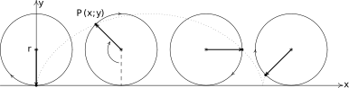
Our goal is to find parametric equations for the coordinates of the point $P (x, y)$ in terms of $θ$ . From our work in Example 14.5.4 number, we know that clockwise motion along the Unit Circle starting at the point $open parenthesis 0, minus 1 close parenthesis$ can be modeled by the equations ${x = - \sin (θ), y = - \cos (θ)$ for $0 less than or equal to θ less than 2 ⁢ π$ . (We have renamed the parameter ` $θ$ ' to match the context of this problem.)

To model this motion on a circle of radius $r$ , all we need to do¹⁰ is multiply both $x$ and $y$ by the factor $r$ which yields ${x = - r \sin (θ), y = - r \cos (θ)$ .

Next, we adjust for the fact that the circle isn't stationary with center $open parenthesis 0, 0 close parenthesis$ , but rather, is rolling along the positive $x$ -axis. Since the velocity $v$ is constant, we know that at time $t$ , the center of the circle has traveled a distance $v t$ down the positive $x$ -axis. Furthermore, since the radius of the circle is $r$ and the circle isn't moving vertically, we know that the center of the circle is always $r$ units above the $x$ -axis. Putting these two facts together, we have that at time $t$ , the center of the circle is at the point $(v t, r)$ .

From Section 11.1.1, we know $v = \frac{r θ}{t}$ , or $v t = r θ$ . Hence, the center of the circle, in terms of the parameter $θ$ , is $(r θ, r)$ . As a result, we need to modify the equations ${x = - r \sin (θ), y = - r \cos (θ)$ by shifting the $x$ -coordinate to the right $r θ$ units (by adding $r θ$ to the expression for $x$ ) and the $y$ -coordinate up $r$ units¹¹ (by adding $r$ to the expression for $y$ ).

We get ${x = - r \sin (θ) + r θ, y = - r \cos (θ) + r$ , which can be written as ${x = r (θ - \sin (θ)), y = r (1 - \cos (θ))$ . Since the motion starts at $θ equals 0$ and proceeds indefinitely, we set $θ greater than or equal to 0$ .

We end the section by using technology to graph a cycloid.

Example 5

Find the parametric equations of a cycloid which results from a circle of radius $3$ rolling down the positive $x$ -axis as described above. Graph your answer using a graphing utility.

We have $r equals 3$ which gives the equations ${x = 3 (t - \sin (t)), y = 3 (1 - \cos (t))$ for $t greater than or equal to 0$ . (Here we have returned to the convention of using $t$ as the parameter.)

Sketching the cycloid by hand is a wonderful exercise in Calculus, but for the purposes of this book, we use a graphing utility. Below is the graph of this cycloid created by desmos .

Figure 14.222

We see the equations create a series of `arches' and can (partially) verify the reasonableness the graph by finding the $x$ -intercepts. To do this, we set $y = 3 (1 - \cos (t)) = 0$ , which amounts to solving $cos ⁡ open parenthesis t close parenthesis equals 1$ .

We get $t equals 2 ⁢ π ⁢ k$ and since $t greater than or equal to 0$ , $k$ can be any nonnegative integer. Substituting a few of these values for $t$ , $t equals 0$ , $t equals 2 ⁢ π$ , $t equals 4 ⁢ π$ , and $t equals 6 ⁢ π$ into the equations $x = 3 (t - \sin (t))$ and $y = 3 (1 - \cos (t))$ we obtain the points $open parenthesis 0, 0 close parenthesis$ , $open parenthesis 6 ⁢ π, 0 close parenthesis approximately equals open parenthesis 18.85, 0 close parenthesis$ , $open parenthesis 12 ⁢ π, 0 close parenthesis approximately equals open parenthesis 37.70, 0 close parenthesis$ and $open parenthesis 18 ⁢ π, 0 close parenthesis approximately equals open parenthesis 56.55, 0 close parenthesis$ , which match the graph. In general, the $x$ -intercepts are $open parenthesis 6 ⁢ π ⁢ k, 0 close parenthesis$ for nonnegative integers $k$ . We leave the details to the reader.

We note it is also possible to analytically determine the (local) maximums of the graph using the techniques demonstrated in Example 14.5.2 by analyzing $y = 3 (1 - \cos (t))$ . The maximums occur when $t = (2 k + 1) π k$ where $k$ is a nonnegative integer, which isn't too surprising just looking at the problem from a symmetry perspective. Substituting these values for $t$ into our equations for $x$ and $y$ produce points of the form $open parenthesis 3 ⁢ open parenthesis 2 ⁢ k plus 1 close parenthesis ⁢ π, 6 close parenthesis$ . We leave the details to the reader.

Exercises

In Exercises -, plot the set of parametric equations by hand. Be sure to indicate the orientation imparted on the curve by the parametrization.

${\begin{matrix} x = 4 t - 3 \\ y = 6 t - 2 \end{matrix} for 0 \leq t \leq 1$
${\begin{matrix} x = 4 t - 1 \\ y = 3 - 4 t \end{matrix} for 0 \leq t \leq 1$
${\begin{matrix} x = 2 t \\ y = t^{2} \end{matrix} for - 1 \leq t \leq 2$
${\begin{matrix} x = t - 1 \\ y = 3 + 2 t - t^{2} \end{matrix} for 0 \leq t \leq 3$
${\begin{matrix} x = t^{2} + 2 t + 1 \\ y = t + 1 \end{matrix} for t \leq 1$
${\begin{matrix} x = \frac{1}{9} (18 - t^{2}) \\ y = \frac{1}{3} t \end{matrix} for t \geq - 3$
${\begin{matrix} x = t \\ y = t^{3} \end{matrix} for - \infty < t < \infty$
${\begin{matrix} x = t^{3} \\ y = t \end{matrix} for - \infty < t < \infty$
${\begin{matrix} x = \cos (t) \\ y = \sin (t) \end{matrix} for - \frac{π}{2} \leq t \leq \frac{π}{2}$
${\begin{matrix} x = 3 \cos (t) \\ y = 3 \sin (t) \end{matrix} for 0 \leq t \leq π$
${\begin{matrix} x = - 1 + 3 \cos (t) \\ y = 4 \sin (t) \end{matrix} for 0 \leq t \leq 2 π$
${\begin{matrix} x = 3 \cos (t) \\ y = 2 \sin (t) + 1 \end{matrix} for \frac{π}{2} \leq t \leq 2 π$
${\begin{matrix} x = 2 \cos (t) \\ y = \sec (t) \end{matrix} for 0 \leq t < \frac{π}{2}$
${\begin{matrix} x = 2 \tan (t) \\ y = \cot (t) \end{matrix} for 0 < t < \frac{π}{2}$
${\begin{matrix} x = \sec (t) \\ y = \tan (t) \end{matrix} for - \frac{π}{2} < t < \frac{π}{2}$
${\begin{matrix} x = \sec (t) \\ y = \tan (t) \end{matrix} for \frac{π}{2} < t < \frac{3 π}{2}$
${\begin{matrix} x = \tan (t) \\ y = 2 \sec (t) \end{matrix} for - \frac{π}{2} < t < \frac{π}{2}$
${\begin{matrix} x = \tan (t) \\ y = 2 \sec (t) \end{matrix} for \frac{π}{2} < t < \frac{3 π}{2}$
${\begin{matrix} x = \cos (t) \\ y = t \end{matrix} for 0 \leq t \leq π$
${\begin{matrix} x = \sin (t) \\ y = t \end{matrix} for - \frac{π}{2} \leq t \leq \frac{π}{2}$

In the same way (and for the same reason) we took the time on page in Section 14.2 to show how to graph polar equations using a graphing calculator, we take a few moments here to explain how to graph a system of parametric equations using a calculator. Our task is to graph the cycloid from Example 14.5.5, ${x = 3 (t - \sin (t)), y = 3 (1 - \cos (t))$ for $t greater than or equal to 0$ using a graphing calculator.

We first must ensure that the calculator is in `Parametric Mode' and `radian mode' when we enter the equations and advance to the `Window' screen.

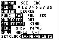
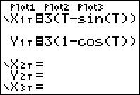
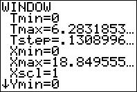
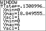
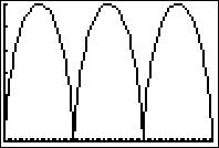
Our next step is to find appropriate bounds on the parameter, $t$ , as well as for $x$ and $y$ . We know that one full revolution of the circle occurs over the interval $0 less than or equal to t less than 2 ⁢ π$ , so it seems reasonable to keep these as our bounds on $t$ . The `Tstep' seems reasonably small – too large a value here can lead to incorrect graphs.¹² We know from our derivation of the equations of the cycloid that the center of the generating circle has coordinates $open parenthesis r ⁢ θ, r close parenthesis equals open parenthesis 3 ⁢ t, 3 close parenthesis$ . Since $t$ ranges between $0$ and $2 ⁢ π$ , we set $x$ to range between $0$ and $6 ⁢ π$ . The values of $y$ go from the bottom of the circle to the top, so $y$ ranges between $0$ and $6$ .

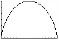
Below we graph the cycloid with these settings, and then extend $t$ to range from $0$ to $6 ⁢ π$ which forces $x$ to range from $0$ to $18 ⁢ π$ yielding three arches of the cycloid.¹³

In Exercises -, plot the set of parametric equations with the help of a graphing utility. Be sure to indicate the orientation imparted on the curve by the parametrization.

${\begin{matrix} x = t^{3} - 3 t \\ y = t^{2} - 4 \end{matrix} for - 2 \leq t \leq 2$
${\begin{matrix} x = 4 \cos^{3} (t) \\ y = 4 \sin^{3} (t) \end{matrix} for 0 \leq t \leq 2 π$
${\begin{matrix} x = e^{t} + e^{- t} \\ y = e^{t} - e^{- t} \end{matrix} for - 2 \leq t \leq 2$
${\begin{matrix} x = \cos (3 t) \\ y = \sin (4 t) \end{matrix} for 0 \leq t \leq 2 π$

In Exercises -, find a parametric description for the given oriented curve.

the directed line segment from $open parenthesis 3, minus 5 close parenthesis$ to $open parenthesis minus 2, 2 close parenthesis$
the directed line segment from $(- 2, - 1)$ to $open parenthesis 3, minus 4 close parenthesis$
the curve $y = 4 - x^{2}$ from $open parenthesis minus 2, 0 close parenthesis$ to $open parenthesis 2, 0 close parenthesis$ .
the curve $y = 4 - x^{2}$ from $open parenthesis minus 2, 0 close parenthesis$ to $open parenthesis 2, 0 close parenthesis$ (Shift the parameter so $t equals 0$ corresponds to $open parenthesis minus 2, 0 close parenthesis$ .)
the curve $x = y^{2} - 9$ from $(- 5, - 2)$ to $open parenthesis 0, 3 close parenthesis$ .
the curve $x = y^{2} - 9$ from $open parenthesis 0, 3 close parenthesis$ to $(- 5, - 2)$ . (Shift the parameter so $t equals 0$ corresponds to $open parenthesis 0, 3 close parenthesis$ .)
the circle $x^{2} + y^{2} = 25$ , oriented counter-clockwise
the circle ${(x - 1)}^{2} + y^{2} = 4$ , oriented counter-clockwise
the circle $x^{2} + y^{2} - 6 y = 0$ , oriented counter-clockwise
the circle $x^{2} + y^{2} - 6 y = 0$ , oriented clockwise (Shift the parameter so $t$ begins at $0$ .)
the circle ${(x - 3)}^{2} + {(y + 1)}^{2} = 117$ , oriented counter-clockwise
the ellipse ${(x - 1)}^{2} + 9 y^{2} = 9$ , oriented counter-clockwise
the ellipse $9 x^{2} + 4 y^{2} + 24 y = 0$ , oriented counter-clockwise
the ellipse $9 x^{2} + 4 y^{2} + 24 y = 0$ , oriented clockwise (Shift the parameter so $t equals 0$ corresponds to $open parenthesis 0, 0 close parenthesis$ .)
the triangle with vertices $open parenthesis 0, 0 close parenthesis$ , $open parenthesis 3, 0 close parenthesis$ , $open parenthesis 0, 4 close parenthesis$ , oriented counter-clockwise (Shift the parameter so $t equals 0$ corresponds to $open parenthesis 0, 0 close parenthesis$ .)
Use parametric equations and a graphing utility to graph the inverse of $f (x) = x^{3} + 3 x - 4$ .
Every polar curve $r = f (θ)$ can be translated to a system of parametric equations with parameter $θ$ by ${x = r \cos (θ) = f (θ) \cos (θ), y = r \sin (θ) = f (θ) \sin (θ)$ . Convert $r equals 6 ⁢ cos ⁡ open parenthesis 2 ⁢ θ close parenthesis$ to a system of parametric equations. Check your answer by graphing $r equals 6 ⁢ cos ⁡ open parenthesis 2 ⁢ θ close parenthesis$ by hand using the techniques presented in Section 14.2 and then graphing the parametric equations you found using a graphing utility.
Use your results from Exercises and in Section 11.3.1 to find the parametric equations which model a passenger's position as they ride the London Eye .

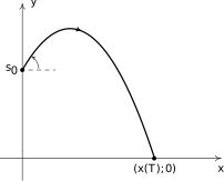
Suppose an object, called a projectile, is launched into the air. Ignoring everything except the force gravity, the path of the projectile is given by¹⁴

${\begin{matrix} x = v_{0} \cos (θ) t \\ y = - \frac{1}{2} g t^{2} + v_{0} \sin (θ) t + s_{0} \end{matrix} for 0 \leq t \leq T$

where $v sub 0$ is the initial speed of the object, $θ$ is the angle from the horizontal at which the projectile is launched,¹⁵ $g$ is the acceleration due to gravity, $s sub 0$ is the initial height of the projectile above the ground and $T$ is the time when the object returns to the ground. (See the figure below.)

Carl's friend Jason competes in Highland Games Competitions across the country. In one event, the `hammer throw', he throws a 56 pound weight for distance. If the weight is released $6$ feet above the ground at an angle of $42 degrees$ with respect to the horizontal with an initial speed of $33$ feet per second, find the parametric equations for the flight of the hammer. (Here, use $g = 32 \frac{ft.}{s^{2}}$ .) When will the hammer hit the ground? How far away will it hit the ground? Check your answer using a graphing utility.
Eliminate the parameter in the equations for projectile motion to show that the path of the projectile follows the curve
$y = - \frac{g \sec^{2} (θ)}{2 v_{0}^{2}} x^{2} + \tan (θ) x + s_{0}$
Use the vertex formula (Equation 1.2) to show the maximum height of the projectile is
$y = \frac{v_{0}^{2} \sin^{2} (θ)}{2 g} + s_{0} when x = \frac{v_{0}^{2} \sin (2 θ)}{2 g}$
In another event, the `sheaf toss', Jason throws a 20 pound weight for height. If the weight is released 5 feet above the ground at an angle of $85 degrees$ with respect to the horizontal and the sheaf reaches a maximum height of 31.5 feet, use your results from part to determine how fast the sheaf was launched into the air. (Once again, use $g = 32 \frac{ft.}{s^{2}}$ .)
Suppose $θ = \frac{π}{2}$ . (The projectile was launched vertically.) Simplify the general parametric formula given for $y (t)$ above using $g = 9.8 \frac{m}{s^{2}}$ and compare that to the formula for $s (t)$ given in Exercise in Section 1.4. What is $x (t)$ in this case?
If $f$ and $g$ are functions, explain why the function $\vec{r} (t) = ⟨ f (t), g (t) ⟩$ is a function. The function $\vec{r}$ is called a vector-valued function since it matches real number inputs, $t$ , with vector outputs, $\vec{r} (t)$ . Explain why when the vectors $\vec{r} (t)$ are plotted in standard position, their terminal points trace out the curve described parametrically by the system of equations: ${x = f (t) y = g (t)$ (In Calculus, you will see systems of parametric equations `packaged' together using vectors.)

In Exercises -, we explore the hyperbolic cosine function, denoted $\cosh (t)$ , and the hyperbolic sine function, denoted $\sinh (t)$ , defined below:

$\begin{matrix} \cosh (t) = \frac{e^{t} + e^{- t}}{2} & and & \sinh (t) = \frac{e^{t} - e^{- t}}{2} \end{matrix}$

Using a graphing utility as needed, verify the following:
1. the domain of $\cosh (t)$ is $open parenthesis minus ∞, ∞ close parenthesis$ and the range of $\cosh (t)$ is $open bracket 1, ∞ close parenthesis$ .
2. the domain and range of $\sinh (t)$ are both $open parenthesis minus ∞, ∞ close parenthesis$ .
Show that ${x (t) = \cosh (t), y (t) = \sinh (t)$ parametrize the right half of the `unit' hyperbola $x^{2} - y^{2} = 1$ . (Hence the use of the adjective `hyperbolic.')
Compare and contrast the definitions of $\cosh (t)$ and $\sinh (t)$ to the formulas for $\cos (t)$ and $\sin (t)$ given in Exercise in Section 14.3.
Four other hyperbolic functions are waiting to be defined: the hyperbolic secant $sech (t)$ , the hyperbolic cosecant $csch (t)$ , the hyperbolic tangent $\tanh (t)$ and the hyperbolic cotangent $\coth (t)$ . Define these functions in terms of $\cosh (t)$ and $\sinh (t)$ , then convert them to formulas involving $e^{t}$ and $e^{- t}$ . Consult a suitable reference (a Calculus book, or this entry on the hyperbolic functions ) and spend some time reliving the thrills of trigonometry with these `hyperbolic' functions.
If these functions look familiar, they should. Enjoy some nostalgia and revisit Exercise in Section 7.6, Exercise in Section 7.4 and the answer to Exercise in Section 7.5.

Answers

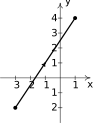
${\begin{matrix} x = 4 t - 3 \\ y = 6 t - 2 \end{matrix} for 0 \leq t \leq 1$
Figure 14.230
${\begin{matrix} x = 4 t - 1 \\ y = 3 - 4 t \end{matrix} for 0 \leq t \leq 1$
Figure 14.231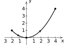
${\begin{matrix} x = 2 t \\ y = t^{2} \end{matrix} for - 1 \leq t \leq 2$
Figure 14.232
${\begin{matrix} x = t - 1 \\ y = 3 + 2 t - t^{2} \end{matrix} for 0 \leq t \leq 3$
Figure 14.233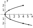
${\begin{matrix} x = t^{2} + 2 t + 1 \\ y = t + 1 \end{matrix} for t \leq 1$
Figure 14.234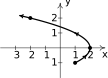
${\begin{matrix} x = \frac{1}{9} (18 - t^{2}) \\ y = \frac{1}{3} t \end{matrix} for t \geq - 3$
Figure 14.235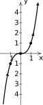
${\begin{matrix} x = t \\ y = t^{3} \end{matrix} for - \infty < t < \infty$
Figure 14.236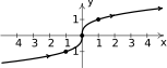
${\begin{matrix} x = t^{3} \\ y = t \end{matrix} for - \infty < t < \infty$
Figure 14.237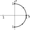
${\begin{matrix} x = \cos (t) \\ y = \sin (t) \end{matrix} for - \frac{π}{2} \leq t \leq \frac{π}{2}$
Figure 14.238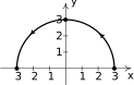
${\begin{matrix} x = 3 \cos (t) \\ y = 3 \sin (t) \end{matrix} for 0 \leq t \leq π$
Figure 14.239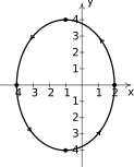
${\begin{matrix} x = - 1 + 3 \cos (t) \\ y = 4 \sin (t) \end{matrix} for 0 \leq t \leq 2 π$
Figure 14.240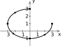
${\begin{matrix} x = 3 \cos (t) \\ y = 2 \sin (t) + 1 \end{matrix} for \frac{π}{2} \leq t \leq 2 π$
Figure 14.241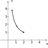
${\begin{matrix} x = 2 \cos (t) \\ y = \sec (t) \end{matrix} for 0 \leq t < \frac{π}{2}$
Figure 14.242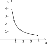
${\begin{matrix} x = 2 \tan (t) \\ y = \cot (t) \end{matrix} for 0 < t < \frac{π}{2}$
Figure 14.243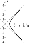
${\begin{matrix} x = \sec (t) \\ y = \tan (t) \end{matrix} for - \frac{π}{2} < t < \frac{π}{2}$
Figure 14.244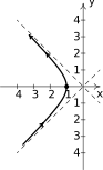
${\begin{matrix} x = \sec (t) \\ y = \tan (t) \end{matrix} for \frac{π}{2} < t < \frac{3 π}{2}$
Figure 14.245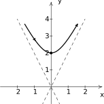
${\begin{matrix} x = \tan (t) \\ y = 2 \sec (t) \end{matrix} for - \frac{π}{2} < t < \frac{π}{2}$
Figure 14.246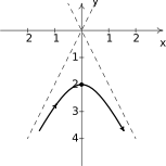
${\begin{matrix} x = \tan (t) \\ y = 2 \sec (t) \end{matrix} for \frac{π}{2} < t < \frac{3 π}{2}$
Figure 14.247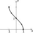
${\begin{matrix} x = \cos (t) \\ y = t \end{matrix} for 0 < t < π$
Figure 14.248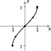
${\begin{matrix} x = \sin (t) \\ y = t \end{matrix} for - \frac{π}{2} < t < \frac{π}{2}$
Figure 14.249
${\begin{matrix} x = t^{3} - 3 t \\ y = t^{2} - 4 \end{matrix} for - 2 \leq t \leq 2$
Figure 14.250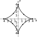
${\begin{matrix} x = 4 \cos^{3} (t) \\ y = 4 \sin^{3} (t) \end{matrix} for 0 \leq t \leq 2 π$
Figure 14.251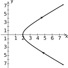
${\begin{matrix} x = e^{t} + e^{- t} \\ y = e^{t} - e^{- t} \end{matrix} for - 2 \leq t \leq 2$
Figure 14.252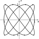
${\begin{matrix} x = \cos (3 t) \\ y = \sin (4 t) \end{matrix} for 0 \leq t \leq 2 π$
Figure 14.253
${\begin{matrix} x = 3 - 5 t \\ y = - 5 + 7 t \end{matrix} for 0 \leq t \leq 1$
${\begin{matrix} x = 5 t - 2 \\ y = - 1 - 3 t \end{matrix} for 0 \leq t \leq 1$
${\begin{matrix} x = t \\ y = 4 - t^{2} \end{matrix} for - 2 \leq t \leq 2$
${\begin{matrix} x = t - 2 \\ y = 4 t - t^{2} \end{matrix} for 0 \leq t \leq 4$
${\begin{matrix} x = t^{2} - 9 \\ y = t \end{matrix} for - 2 \leq t \leq 3$
${\begin{matrix} x = t^{2} - 6 t \\ y = 3 - t \end{matrix} for 0 \leq t \leq 5$
${\begin{matrix} x = 5 \cos (t) \\ y = 5 \sin (t) \end{matrix} for 0 \leq t < 2 π$
${\begin{matrix} x = 1 + 2 \cos (t) \\ y = 2 \sin (t) \end{matrix} for 0 \leq t < 2 π$
${\begin{matrix} x = 3 \cos (t) \\ y = 3 + 3 \sin (t) \end{matrix} for 0 \leq t < 2 π$
${\begin{matrix} x = 3 \cos (t) \\ y = 3 - 3 \sin (t) \end{matrix} for 0 \leq t < 2 π$
${\begin{matrix} x = 3 + \sqrt{117} \cos (t) \\ y = - 1 + \sqrt{117} \sin (t) \end{matrix} for 0 \leq t < 2 π$
${\begin{matrix} x = 1 + 3 \cos (t) \\ y = \sin (t) \end{matrix} for 0 \leq t < 2 π$
${\begin{matrix} x = 2 \cos (t) \\ y = 3 \sin (t) - 3 \end{matrix} for 0 \leq t < 2 π$
${\begin{matrix} x = 2 \cos (t - \frac{π}{2}) = 2 \sin (t) \\ y = - 3 - 3 \sin (t - \frac{π}{2}) = - 3 + 3 \cos (t) \end{matrix} for 0 \leq t < 2 π$
${x (t), y (t)$ where:
$\begin{matrix} x (t) = {\begin{matrix} 3 t, & 0 \leq t \leq 1 \\ 6 - 3 t, & 1 \leq t \leq 2 \\ 0, & 2 \leq t \leq 3 \end{matrix} & y (t) = {\begin{matrix} 0, & 0 \leq t \leq 1 \\ 4 t - 4, & 1 \leq t \leq 2 \\ 12 - 4 t, & 2 \leq t \leq 3 \end{matrix} \end{matrix}$
The parametric equations for the inverse are ${\begin{matrix} x = t^{3} + 3 t - 4 \\ y = t \end{matrix} for - \infty < t < \infty$
$r equals 6 ⁢ cos ⁡ open parenthesis 2 ⁢ θ close parenthesis$ translates to ${\begin{matrix} x = 6 \cos (2 θ) \cos (θ) \\ y = 6 \cos (2 θ) \sin (θ) \end{matrix} for 0 \leq θ < 2 π$ .
The parametric equations which describe the locations of passengers on the London Eye are
${\begin{matrix} x = 67.5 \cos (\frac{π}{15} t - \frac{π}{2}) = 67.5 \sin (\frac{π}{15} t) \\ y = 67.5 \sin (\frac{π}{15} t - \frac{π}{2}) + 67.5 = 67.5 - 67.5 \cos (\frac{π}{15} t) \end{matrix} for - \infty < t < \infty$
The parametric equations for the hammer throw are ${\begin{matrix} x = 33 \cos (42^{\circ}) t \\ y = - 16 t^{2} + 33 \sin (42^{\circ}) t + 6 \end{matrix}$ for $t greater than or equal to 0$ .
To find when the hammer hits the ground, we solve $y ⁢ open parenthesis t close parenthesis equals 0$ and get $t \approx - 0.23$ or $1.61$ . Since $t greater than or equal to 0$ , the hammer hits the ground after approximately $t equals 1.61$ seconds after it was launched into the air.
To find how far away the hammer hits the ground, we find $x ⁢ open parenthesis 1.61 close parenthesis approximately equals 39.48$ feet from where it was thrown into the air.
We solve $y = \frac{v_{0}^{2} \sin^{2} (θ)}{2 g} + s_{0} = \frac{v_{0}^{2} \sin^{2} (85^{\circ})}{2 (32)} + 5 = 31.5$ to get $v_{0} = \pm 41.34$ .
The initial speed of the sheaf was approximately $41.34$ feet per second.

Note the use of the indefinite article `a'. As we shall see, there are infinitely many different parametric representations for any given curve. ↩
Here, the bug reaches the point $Q$ at two different times. While this does not contradict our claim that $f (t)$ and $g (t)$ are functions of $t$ , it shows that neither $f$ nor $g$ can be one-to-one. (Think about this before reading on.) ↩
We will have an example shortly where no matter how we restrict $x$ and $y$ , we can never accurately describe the curve once we've eliminated the parameter. ↩
You should review Definitions 1.7 and 2.7 if you've forgotten what `increasing', `decreasing' and `local minimum' mean. ↩
The reader is encouraged to review Sections 7.2 and 7.3 as needed. ↩
Note the open circle at the origin. See our discussion about holes in graphs in Example 1.1.6 in Section 1.1. ↩
See the discussion preceding Example 5.5.4 in Section 5.5 for a review of this concept. ↩
Provided you followed the inverse function theory, of course. ↩
Compare and contrast this with Exercise in Section 13.3. ↩
If we replace $x$ with $\frac{x}{r}$ and $y$ with $\frac{y}{r}$ in the equation for the Unit Circle $x^{2} + y^{2} = 1$ , we obtain ${(\frac{x}{r})}^{2} + {(\frac{y}{r})}^{2} = 1$ which reduces to $x^{2} + y^{2} = r^{2}$ . In the language of Section 5.4, we are stretching the graph by a factor of $r$ in both the $x$ - and $y$ -directions. Hence, we multiply both the $x$ - and $y$ -coordinates of points on the graph by $r$ . ↩
Does this seem familiar? See Example 11.3.4 in Section 11.3.1. ↩
Again, see page in Section 14.2. ↩
It is instructive to note that keeping the $y$ settings between 0 and 6 skews the aspect ratio of the cycloid. Using the `Zoom Square' feature on the graphing calculator gives a true geometric perspective of the three arches. ↩
A nice mix of vectors and Calculus are needed to derive this. ↩
We've seen this before. It's the angle of elevation which was defined on page . ↩

Adapted from Precalculus, Preliminary 4th Edition (integrated calculus), by Carl Stitz and Jeff Zeager (stitz-zeager.com), licensed under CC BY-NC-SA 3.0. Changes were made: reformatted as an accessible XYZ web edition. License: CC-BY-NC-SA-3.0.