Chapter 14: Polar Coordinates and Parametric Equations

In Section A.3, we introduced the notion of assigning ordered pairs of real numbers called `coordinates' to points in the plane. Recall the Cartesian coordinate plane is defined using two number lines – one horizontal and one vertical – which intersect at right angles at a point called the `origin'.

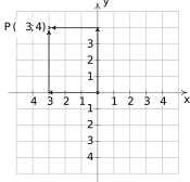
As seen below on the left, to plot a point with Cartesian coordinates, say $P(-3,4)$, we start at the origin, travel horizontally to the left $3$ units, then up $4$ units. Alternatively, we could start at the origin, travel up $4$ units, then to the left $3$ units and arrive at the same location.

For the most part, the `motions' of the Cartesian system (over and up) describe a rectangle, and most points can be thought of as the corner diagonally across the rectangle from the origin. For this reason, the Cartesian coordinates of a point are often called `rectangular' coordinates.

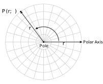
In this section, we introduce a new system for assigning coordinates to points in the plane – polar coordinates as diagrammed above on the right. We start with an origin point, called the pole, and a ray called the polar axis.