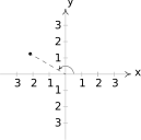
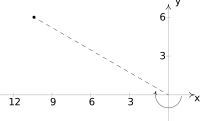
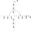
In Section A.3, we introduced the notion of assigning ordered pairs of real numbers called `coordinates' to points in the plane. Recall the Cartesian coordinate plane is defined using two number lines – one horizontal and one vertical – which intersect at right angles at a point called the `origin'.
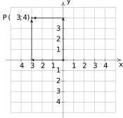
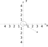
As seen below on the left, to plot a point with Cartesian coordinates, say , we start at the origin, travel horizontally to the left units, then up units. Alternatively, we could start at the origin, travel up units, then to the left units and arrive at the same location.
For the most part, the `motions' of the Cartesian system (over and up) describe a rectangle, and most points can be thought of as the corner diagonally across the rectangle from the origin.1 For this reason, the Cartesian coordinates of a point are often called `rectangular' coordinates.
Figure 14.1Figure 14.2
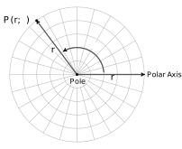
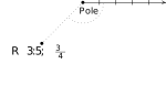
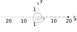
In this section, we introduce a new system for assigning coordinates to points in the plane – polar coordinates as diagrammed above on the right. We start with an origin point, called the pole, and a ray called the polar axis.
We locate a point using two coordinates, , where represents a directed distance from the pole2 and is a measure of counter-clockwise rotation from the polar axis.
Roughly speaking, the polar coordinates of a point measure `how far out' the point is from the pole (that's ), and `how far to rotate' from the polar axis, (that's ).
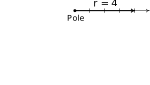
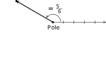
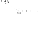
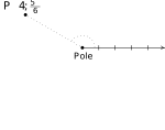
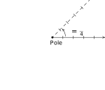
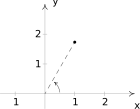
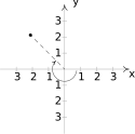
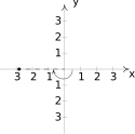
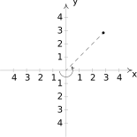
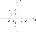
For example, if we wished to plot the point with polar coordinates , we'd start at the pole, move out along the polar axis units, then rotate radians counter-clockwise.
Figure 14.3Figure 14.4Figure 14.5
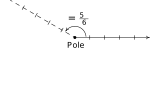
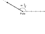
We may also visualize this process by thinking of the rotation first.3 To plot this way, we rotate counter-clockwise from the polar axis, then move outwards from the pole units. Essentially we are locating a point on the terminal side of which is units away from the pole.
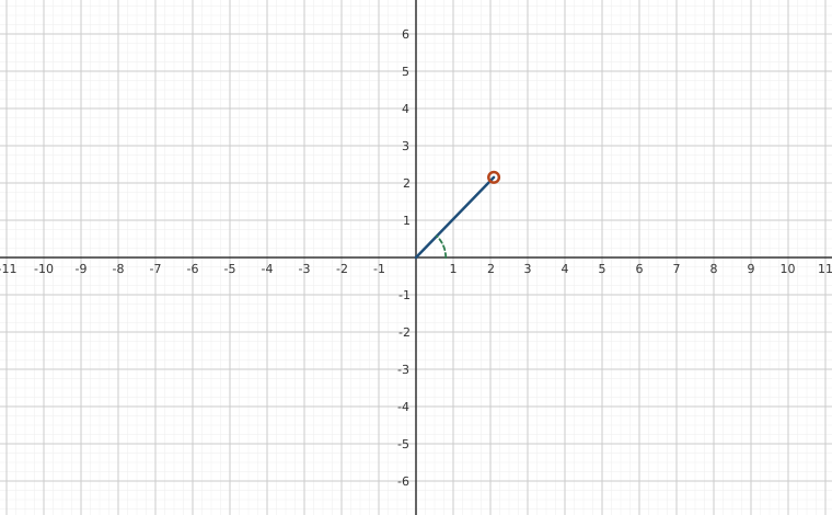
Interactive figurePlotting (r, θ): turn through θ, then walk r units, backwards if r is negativeDrag the Signed distance r and Angle θ (radians) sliders.
XYZ Graph · viewer build 5edf91b
A polar point is reached in two motions: rotate from the positive x-axis through the angle θ, shown by the dashed green arc, then travel r units along that direction, shown by the navy ray ending at the marked point. Slide θ and the ray sweeps around the pole; slide r past zero and the point jumps to the opposite side of the pole, because a negative r means walking backwards along the ray. The same point can be named in infinitely many ways, and the sliders let the reader find several of them.Figure 14.6Figure 14.7Figure 14.8
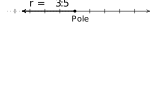
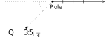
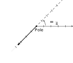
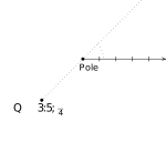
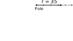
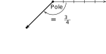
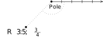
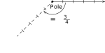
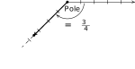
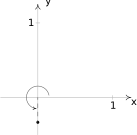
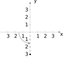
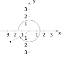
If , we begin by moving in the opposite direction on the polar axis from the pole. For example, to plot the point with polar coordinates we have
Figure 14.9Figure 14.10Figure 14.11
If we interpret the angle first, we rotate radians, then move back through the pole units. Here we are locating a point units away from the pole on the terminal side of , not .
Figure 14.12Figure 14.13Figure 14.14
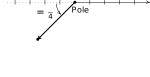
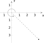
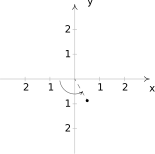
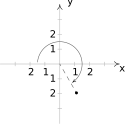
As you may have guessed, means the rotation away from the polar axis is clockwise instead of counter-clockwise. Hence, to plot we have the following.
Figure 14.15Figure 14.16Figure 14.17
From an `angles first' approach, we rotate then move out units from the pole. We see that is the point on the terminal side of which is units from the pole.
Figure 14.18Figure 14.19Figure 14.20
The points and above are, in fact, the same point despite the fact that their polar coordinate representations are different. Unlike Cartesian coordinates where and represent the same point if and only if and , a point can be represented by infinitely many polar coordinate pairs.
We explore this notion more in the following example.
In light of our work in Example 14.1.1, it should come as no surprise that any given point expressed in polar coordinates has infinitely many other representations in polar coordinates.
The following result characterizes when two sets of polar coordinates determine the same point in the plane. It could be considered as a definition or a theorem, depending on your point of view. We choose to state it as a property of the polar coordinate system.
Equivalent Representations of Points in Polar Coordinates
Suppose and are polar coordinates where , and the angles are measured in radians. Then and determine the same point if and only if one of the following is true:
and for some integer
and for some integer
All polar coordinates of the form represent the pole regardless of the value of .
The key to understanding this result, and indeed the whole polar coordinate system, is to keep in mind that means .
If , then no matter how much rotation is performed, the point never leaves the pole. Thus is the pole for all values of .
Now let's assume that neither nor is zero. If and determine the same point then the (non-zero) distance from to the pole in each case must be the same. Since this distance is controlled by the first coordinate, we have that either or .
If , then when plotting and , the angles and have the same initial side. Hence, if and determine the same point, we must have that is coterminal with . We know that this means for some integer , as required.
If, on the other hand, , then when plotting and , the initial side of is rotated radians away from the initial side of . In this case, must be coterminal with . Hence, which we rewrite as for some integer .
Conversely, if and for some integer , then the points and lie the same (directed) distance from the pole on the terminal sides of coterminal angles, and hence are the same point.
Now suppose and for some integer . To plot , we first move a directed distance from the pole; to plot , our first step is to move the same distance from the pole as , but in the opposite direction. At this intermediate stage, we have two points equidistant from the pole rotated exactly radians apart. Since for some integer , we see that is coterminal to and it is this extra radians of rotation which aligns the points and .
Next, we marry the polar coordinate system with the Cartesian (rectangular) coordinate system. To do so, we identify the pole and polar axis in the polar system to the origin and positive -axis, respectively, in the rectangular system. We get the following result.
In the case , Theorem 14.1 is an immediate consequence of Theorems 11.3 and 11.9.
If , then we know an alternate representation for is . Since in this case, , we know the theorem as stated is true for the representation so we apply it here.
Moreover, , and , so the theorem is true in this case, too.
The remaining case is , in which case is the pole. Since the pole is identified with the origin in rectangular coordinates, the theorem in this case amounts to checking `.'
Since we have argued that Theorem 14.1 is true in all cases, we put it to good use in the following example.
Now that we've had practice converting representations of points between the rectangular and polar coordinate systems, we now set about converting equations from one system to another.
Just as we've used equations in and to represent relations in rectangular coordinates (see Section 5.5), equations in the variables and represent relations in polar coordinates. We convert equations between the two systems using Theorem 14.1 as the next example illustrates.
In practice, much of the pedantic verification of the equivalence of equations in Example 14.1.3 is left unsaid. Indeed, in most textbooks, squaring equations like to arrive at happens without a second thought. Your instructor will ultimately decide how much, if any, justification is warranted.
If you take anything away from Example 14.1.3, it should be that relatively simple equations in rectangular coordinates, such as , can become quite complicated in polar coordinates, and vice-versa.
In the next section, we devote our attention to graphing equations like the ones given in Example 14.1.3 number on the Cartesian coordinate plane without converting back to rectangular coordinates. If nothing else, number above shows the price we pay if we insist on always converting to back to the more familiar rectangular coordinate system.
Exercises
In Exercises -, plot the point given in polar coordinates and then give three different expressions for the point such that (a) and , (b) and (c) and
In Exercises -, convert the point from polar coordinates into rectangular coordinates.
In Exercises -, plot each point given in rectangular coordinates and convert to polar coordinates. Choose and .
In Exercises -, convert the equation from rectangular coordinates into polar coordinates. Solve for in all but through. In Exercises -, solve for
In Exercises -, convert the equation from polar coordinates into rectangular coordinates.
Convert the origin into polar coordinates in four different ways.
With the help of your classmates, use the Law of Cosines to develop a formula for the distance between two points in polar coordinates.
Answers
Figure 14.41
Figure 14.42
Figure 14.43
Figure 14.44
Figure 14.45
Figure 14.46
Figure 14.47
Figure 14.48
Figure 14.49
Figure 14.50
Figure 14.51
Figure 14.52
Figure 14.53
Figure 14.54
Figure 14.55
Figure 14.56
or
or
or
or
Any point of the form will work, e.g. and
Adapted from Precalculus with Integrated Calculus, edition 4i, by Carl Stitz and Jeff Zeager (stitz-zeager.com), licensed under CC BY-NC-SA 3.0. Changes were made: reformatted as an accessible XYZ web edition. License: CC-BY-NC-SA-3.0.
These eBooks are a prerelease and are not yet certified conformant with WCAG 2.1 AA or any other accessibility standard. Every page is built against an automated accessibility gate, and our target for the published editions is WCAG 2.2 Level AA. If something is unusable, please tell us.