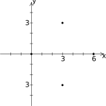
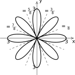
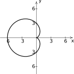
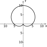
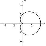
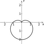
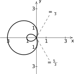
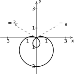
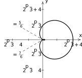
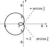
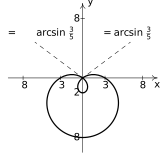
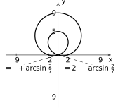
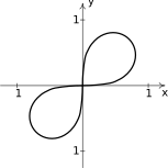
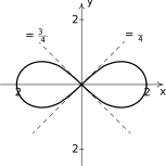
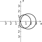
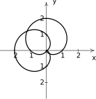
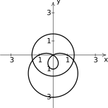
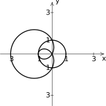
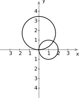
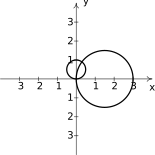
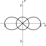
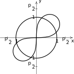
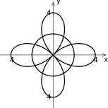
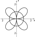
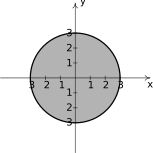
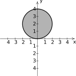
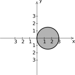
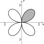
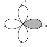
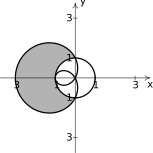
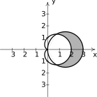
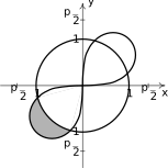
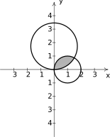
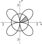
In this section, we discuss how to graph equations relating the polar coordinate variables and on the rectangular coordinate plane. Since every point in the plane has infinitely many different representations in polar coordinates, in order for a point to be on the graph of a given equation, there must be at least one representation of that satisfies that equation.
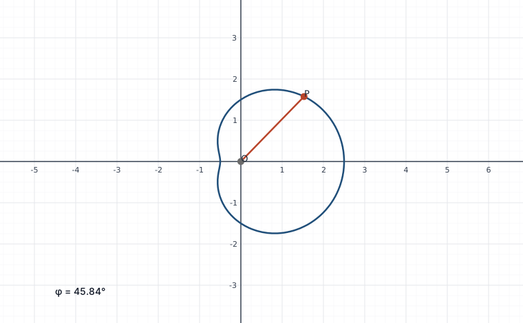
Interactive figureA limaçon r = a + cos θ, swept by the angleDrag O; move the Shape parameter a and Sweep angle φ sliders.
The polar curve r = a + cos θ drawn on the rectangular plane, with two sliders: a reshapes the curve — an inner loop for a < 1, a cardioid's cusp at a = 1, a dimple for 1 < a < 2, and a convex oval beyond — while φ sweeps a radius from the origin to the point of the curve at angle φ. The segment's length is r(φ) = a + cos φ; watch it shrink through zero when a < 1 and φ passes the angles where cos φ = −a, which is exactly where the inner loop is traced.
In our first example, only one of the variables and is present making the other variable free.1 This makes these graphs easier to visualize than others.
Hopefully, our experience in Example 14.2.1 makes the following result clear.
Suppose we wish to graph . A reasonable way to start is to treat as the independent variable, as the dependent variable, evaluate at some `friendly' values of and plot the resulting points.2
Figure 14.65
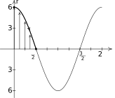
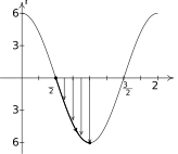
Despite having nine ordered pairs, we get only four distinct points on the graph. For this reason, we employ a slightly different strategy. We graph one cycle of on the -plane3 below on the left and use it to help graph the equation on the -plane below on the right.
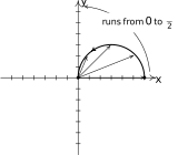
We see that as ranges from to , ranges from to . In the -plane, this means that the curve starts units from the origin on the positive -axis () and gradually returns to the origin by the time the curve reaches the -axis ().
The arrows drawn in the figure below are meant to help you visualize this process. In the -plane, the arrows are drawn from the -axis to the curve . In the -plane, each of these arrows starts at the origin and is rotated through the corresponding angle , in accordance with how we plot polar coordinates. This method is less precise than plotting actual function values, but much faster.
Figure 14.66Figure 14.67
in the -plane
in the -plane
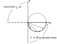
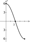
Next, we repeat the process as ranges from to . Here, the values are all negative. This means that in the -plane, instead of graphing in Quadrant II, we graph in Quadrant IV, with all of the angle rotations starting from the negative -axis.
Figure 14.68Figure 14.69
in the -plane
in the -plane
As ranges from to , the values are still negative, which means the graph is traced out in Quadrant I instead of Quadrant III. Since the for these values of match the values for in , we have that the curve begins to retrace itself at this point.
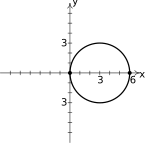
Proceeding further, we find that when , we retrace the portion of the curve in Quadrant IV that we first traced out as . The reader is invited to verify that plotting any range of outside the interval results in retracting some portion of the curve.4 We present the final graph below.
Figure 14.70Figure 14.71
in the -plane
in the -plane
A few remarks are in order. First, there is no relation, in general, between the period of the function and the length of the interval required to sketch the complete graph of in the -plane.
As we saw on page, despite the fact that the period of is , we sketched the complete graph of in the -plane just using the values of as ranged from to .
On the other hand, in Example 14.2.2, number, the period of is , but in order to obtain the complete graph of , we needed to run from to .
Second, the symmetry seen in the examples is also a common occurrence when graphing polar equations.
In addition symmetry about each axis and the origin, it is possible to talk about rotational symmetry with these curves. We leave the exploration of symmetry to Exercises -.
Last we note that while many of the `common' polar graphs can be grouped into families,9 the authors truly feel that taking the time to work through each graph in the manner presented here is the best way to not only understand the polar coordinate system, but also prepare you for what is needed in Calculus.
Next we turn our attention to finding the intersection points of polar curves. What complicates matters in polar coordinates is that any given point has infinitely many representations. As a result, if a point is on the graph of two different polar equations, it is entirely possible that the representation which satisfies one of the equations does not satisfy the other equation.
In our next example, we see the need to rely on Geometry as much as Algebra to solve each problem.
Our work in Example 14.2.3 justifies the following.
Guidelines for Finding Points of Intersection of Graphs of Polar Equations:
To find the points of intersection of the graphs of two polar equations and :
Sketch the graphs of and . Check to see if the curves intersect at the origin (pole).
Solve for pairs which satisfy both and .
Substitute for in either one of or (but not both) and solve for pairs which satisfy both equations. Keep in mind that is an integer.
Substitute for and for in either one of or (but not both) and solve for pairs which satisfy both equations. Keep in mind that is an integer.
Our last example ties together graphing and points of intersection to describe regions in the plane.
Exercises
In Exercises -, plot the graph of the polar equation by hand. Carefully label your graphs.
Circle:
Circle:
Rose:
Rose:
Rose:
Rose:
Rose:
Rose:
Cardioid:
Cardioid:
Cardioid:
Cardioid:
Limaçon:
Limaçon:
Limaçon:
Limaçon:
Limaçon:
Limaçon:
Lemniscate:
Lemniscate:
In Exercises -, find the exact polar coordinates of the points of intersection of graphs of the polar equations. Remember to check for intersection at the pole (origin).
and
and
and
and
and
and
and
and
and
and
In Exercises -, sketch the region in the -plane described by the given set.
In Exercises -, use set-builder notation to describe the polar region. Assume that the region contains its bounding curves.
The region inside the circle .
The region inside the circle which lies in Quadrant III.
The region inside the left half of the circle .
The region inside the circle which lies in Quadrant IV.
The region inside the top half of the cardioid
The region inside the cardioid which lies in Quadrants I and IV.
The inside of the petal of the rose which lies on the positive -axis
The region inside the circle but outside the circle .
The region which lies inside of the circle but outside of the circle
The region in Quadrant I which lies inside both the circle as well as the rose
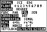
While the authors truly believe that graphing polar curves by hand is fundamental to your understanding of the polar coordinate system, we would be derelict in our duties if we totally ignored the graphing utility.17 Indeed, there are some important polar curves which are simply too difficult to graph by hand and that makes the calculator an important tool for your further studies in Mathematics, Science and Engineering. We now give a brief demonstration of how to use the graphing utility to plot polar curves. The first thing you must do is switch the MODE of your calculator to POL, which stands for “polar”.
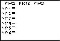
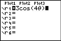
Figure 14.124Figure 14.125Figure 14.126
This changes the “Y=” menu as seen above in the middle. Let's plot the polar rose given by from Exercise above. We type the function into the “r=” menu as seen above on the right. We need to set the viewing window so that the curve displays properly, but when we look at the WINDOW menu, we find three extra lines.
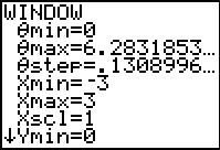
Figure 14.127Figure 14.128
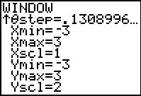
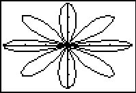
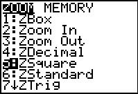
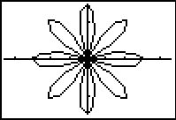
In order for the calculator to be able to plot in the -plane, we need to tell it not only the dimensions which and will assume, but we also what values of to use. From our previous work, we know that we need , so we enter the data you see above. (I'll say more about the -step in just a moment.) Hitting GRAPH yields the curve below on the left which doesn't look quite right. The issue here is that the calculator screen is 96 pixels wide but only 64 pixels tall. To get a true geometric perspective, we need to hit ZOOM SQUARE (seen below in the middle) to produce a more accurate graph which we present below on the right.
Figure 14.129Figure 14.130Figure 14.131
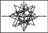
In function mode, the calculator automatically divided the interval [Xmin, Xmax] into 96 equal subintervals. In polar mode, however, we must specify how to split up the interval [min, max] using the step. For most graphs, a step of 0.1 is fine. If you make it too small then the calculator takes a long time to graph. It you make it too big, you get chunky garbage like this.
Figure 14.132
You will need to experiment with the settings in order to get a nice graph. Exercises - give you some curves to graph using your calculator. Note some of them have explicit bounds on and others do not.
Use a graphing utility to graph for various (positive) values of and . Describe the shape of the curve when , , and when .
How many petals does the polar rose have? What about , and ? With the help of your classmates, make a conjecture as to how many petals the polar rose has for any natural number . Replace sine with cosine and repeat the investigation. How many petals does have for each natural number ?
Looking back through the graphs in the section, it's clear that many polar curves enjoy various forms of symmetry. However, classifying symmetry for polar curves is not as straight-forward as it was for equations back in Section 5.5. In Exercises -, we have you and your classmates explore some of the more basic forms of symmetry seen in common polar curves.
Show that if is even18 then the graph of is symmetric about the -axis.
Show that is even and verify that the graph of is indeed symmetric about the -axis. (See Example 14.2.2 number.)
Show that is not even, yet the graph of
is symmetric about the -axis. (See Example 14.2.3 number.)
Show that if is odd19 then the graph of is symmetric about the origin.
Show that is odd and verify that the graph of is indeed symmetric about the origin. (See Example 14.2.2 number.)
Show that is not odd, yet the graph of
is symmetric about the origin. (See Example 14.2.3 number.)
Show that if for all in the domain of then the graph of is symmetric about the -axis.
For , show that and the graph of is symmetric about the -axis, as required. (See Example 14.2.2 number.)
For , show that , yet the graph of
is symmetric about the -axis. (See Example 14.2.2 number.)
In Section 5.4, we discussed transformations of graphs. In Exercise we have you and your classmates explore transformations of polar graphs.
For Exercises and below, let and .
Using a graphing utility, compare the graph of to each of the graphs of , , and . Repeat this process for . In general, how do you think the graph of compares with the graph of ?
Using a graphing utility, compare the graph of to each of the graphs of , , and . Repeat this process for . In general, how do you think the graph of compares with the graph of ?
Follow up question: does it matter if or ?
In light of Exercises -, how would the graph of compare with the graph of for a generic function ? What about the graphs of and ? What about and ? Test out your conjectures using a variety of polar functions found in this section with the help of a graphing utility.
With the help of your classmates, research cardioid microphones.
Answers
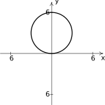
Circle:
Figure 14.133
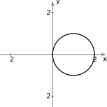
Circle:
Figure 14.134
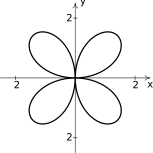
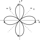
Rose:
Figure 14.135
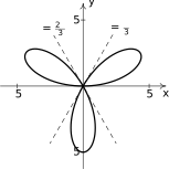
Rose:
Figure 14.136
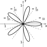
Rose:
Figure 14.137
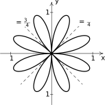
Rose:
Figure 14.138
Rose:
Figure 14.139
Rose:
Figure 14.140
Cardioid:
Figure 14.141
Cardioid:
Figure 14.142
Cardioid:
Figure 14.143
Cardioid:
Figure 14.144
Limaçon:
Figure 14.145
Limaçon:
Figure 14.146
Limaçon:
Figure 14.147
Limaçon:
Figure 14.148
Limaçon:
Figure 14.149
Limaçon:
Figure 14.150
Lemniscate:
Figure 14.151
Lemniscate:
Figure 14.152
and
Figure 14.153
, , pole
and
Figure 14.154
, , pole
and
Figure 14.155
,
and
Figure 14.156
, ,
and
Figure 14.157
, pole
and
Figure 14.158
, pole
and
Figure 14.159
, , ,
and
Figure 14.160
, , ,
and
Figure 14.161
, , ,
, , ,
,
and
Figure 14.162
, , ,
, , ,
,
Figure 14.163
Figure 14.164
Figure 14.165
Figure 14.166
Figure 14.167
Figure 14.168
Figure 14.169
Figure 14.170
Figure 14.171
Figure 14.172
or
or
Adapted from Precalculus with Integrated Calculus, edition 4i, by Carl Stitz and Jeff Zeager (stitz-zeager.com), licensed under CC BY-NC-SA 3.0. Changes were made: reformatted as an accessible XYZ web edition. License: CC-BY-NC-SA-3.0.
These eBooks are a prerelease and are not yet certified conformant with WCAG 2.1 AA or any other accessibility standard. Every page is built against an automated accessibility gate, and our target for the published editions is WCAG 2.2 Level AA. If something is unusable, please tell us.