
11.5 Graphs of Secant, Cosecant, Tangent, and Cotangent Functions
Graphs of the Secant and Cosecant Functions
As mentioned at the end of Section 11.4, one way to proceed with our analysis of the circular functions is to use what we know about the functions and to rewrite the four additional circular functions in terms of sine and cosine with help from Theorem 11.7. We use this approach to analyze .
Rewriting , we first note that is undefined whenever . Thanks to Example 11.2.4 number, we know whenever for integers .
This gives us one way to describe the domain of : . To get a better feel for the set of real numbers we're dealing with, we write out and graph the domain on the number line.
Running through a few values of , we find some of the values excluded from the domain: . Using these we can graph the domain on the number line below.

Expressing this set using interval notation is a bit of a challenge, owing to the infinitely many intervals present. As a first attempt, we have: , where, as usual, the periods of ellipsis indicate the pattern continues indefinitely.1 Hence, for now, it suffices to know that the domain of excludes the odd multiples of .
To find the range of , we find it helpful once again to view . We know the range of is , and since is undefined when , we split our discussion into two cases: when and when .
If , then we can divide the inequality by to obtain . Moreover, we see as , . If, on the other hand, if , then dividing by causes a reversal of the inequality so that . In this case, as , . Since admits all of the values in , the function admits all of the values in .
Since is periodic with period , it shoudn't be too surprising to find that is also. Indeed, provided and are defined, if and only if . Said differently, `inherits' its period from .
We now turn our attention to graphing . Using the table of values we tabulated when graphing in Section 11.3, we can generate points on the graph of by taking reciprocals.
Using the techniques developed in Section 3.1, we can more closely analyze the behavior of near the values excluded from its domain. We find as , , so . Similarly, we get , , and . This means the lines and are vertical asymptotes to the graph of .
Below on the right we graph a fundamental cycle of with the graph of the fundamental cycle of dotted for reference.
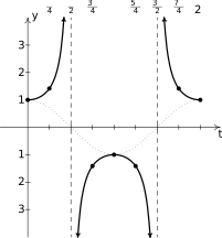
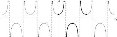
To get a graph of the entire secant function, we paste copies of the fundamental cycle end to end to produce the graph below. The graph suggests that is even. Indeed, since is even, that is, , we have . Hence, along with its period, the secant function inherits its symmetry from the cosine function.
As one would expect, to graph we begin with and take reciprocals of the corresponding -values. Here, we encounter issues at , , , and, in general, at all whole number multiples of , so the domain of is . Not surprisingly, these values produce vertical asymptotes.
Proceeding as above, we graph produce the graph of the fundamental cycle of below along with the dotted graph of for reference.
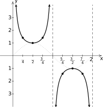
Pasting copies of the fundamental period of end to end produces the graph below. Since the graphs of and are merely phase shifts of each other, it is not too surprising to find the graphs of and are as well.
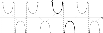
As with the graph of secant, the graph below suggests symmetry. Indeed, since the sine function is odd, that is , so too is the cosecant function: . Hence, the graph of is symmetric about the origin.
Note that, on the intervals between the vertical asymptotes, both and are continuous and smooth. In other words, they are continuous and smooth on their domains.2
The following theorem summarizes the properties of the secant and cosecant functions. Note that all of these properties are direct results of them being reciprocals of the cosine and sine functions, respectively.
In the next example, we discuss graphing more general secant and cosecant curves. We make heavy use of the fact they are reciprocals of sine and cosine functions and apply what we learned in Section 11.3.
As suggested in Example 11.5.1, the concepts of frequency, period, phase shift, and baseline are alive and well with graphs of the secant and cosecant functions. Since the secant and cosecant curves are unbounded, we do not have the concept of `amplitude' for these curves. That being said, the amplitudes of the corresponding cosine and sine curves do play a role here - they measure how wide the gap is between the baseline and the curve.
We gather these observations in the following result whose proof is a consequence of Theorem 11.6 and is relegated to Exercise.
We put Theorem 11.11 to good use in the next example.
We cannot stress enough that our answers to Example 11.5.2 are one of many. For example, in Exercise, we ask you to rework this example choosing . It is well worth the time to think about what relationships exist between the different answers, however. For now, we move on to graphing the last pair of circular functions: tangent and cotangent curves.
Graphs of the Tangent and Cotangent Functions
Next, we turn our attention to the tangent and cotangent functions. Viewing , we find the domain of excludes all values where . Hence, the domain of is . Using this information along with the common values we derived in Section 11.4, we create the table of values below on the left.
Investigating the behavior near the values excluded from the domain, we find as , and . Hence, producing a vertical asymptote to the graph at . Similarly, we get that as , , and .
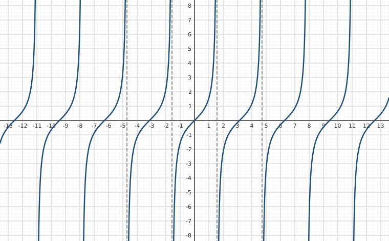
Putting all of this information together, we graph over the interval below on the right.
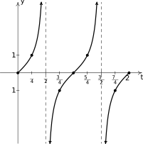
After the usual `copy and paste' procedure, we create the graph of below:
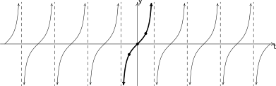
The graph of suggests symmetry through the origin. Indeed, tangent is odd since sine is odd and cosine is even: .
We also see the graph suggests the range of is all real numbers, . We present one proof of this fact in Exercise.
Moreover, as noted in Section 11.4, the period of the tangent function is , and we see that reflected in the graph. This means we can choose any interval of length to serve as our `fundamental cycle.'
We choose the cycle traced out over the (open) interval as highlighted above. In addition to the asymptotes at the endpoints , we use the `quarter marks' and .
It should be no surprise that behaves similarly to . Since , the domain of excludes the values where : .
After analyzing the behavior of near the values excluded from its domain along with plotting points, we graph over the interval below on the right.
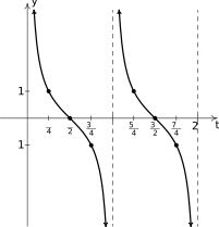
As usual, pasting copies end to end produces the graph of below.
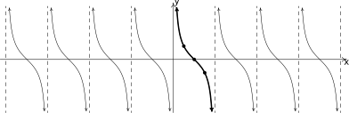
As with , the graph of suggests is odd, a fact we leave to the reader to prove in Exercise. Also, we see that the period of cotangent (like tangent) is and the range is .
We take as one fundamental cycle the graph as traced out over the interval , highlighted above, with quarter marks: , , , and .
The properties of the tangent and cotangent functions are summarized below. As with Theorem 11.10, each of the results below can be traced back to properties of the cosine and sine functions and the definition of the tangent and cotangent functions as quotients thereof.
Unlike the secant and cosecant functions, the tangent and cotangent functions have different periods than sine and cosine. Moreover, in the case of the tangent function, the fundamental cycle we've chosen starts at instead of . Nevertheless, we can use the same notions of period and phase shift to graph transformed versions of tangent and cotangent functions, since these results ultimately trace back to applying Theorem 5.11. We state a version of Theorem 11.6 for tangent and cotangent functions below.
The proof of the proof of Theorem 11.13 is left to the reader in Exercise.
We put Theorem 11.13 to good use in the following example.
Once again, our answers to Example 11.5.4 are one of many, and we invite the reader to think about what all of the solutions would have in common. We close this section with an application.
Extended Interval Notation
Using interval notation to describe the domains of the secant, cosecant, tangent, and cotangent functions is complicated by the fact there are infinitely many intervals to represent. In this section, we introduce extended interval notation to handle these situations.
Let us return to the domain of , . Using interval notation, we describe this set as:
In order to write this set in a more compact way, we let denote the the th real number excluded from the domain. That is, . (This is sequence notation from Chapter 10.)
Getting a common denominator and factoring out the in the numerator, we get . The set we're after consists of the union of intervals determined by the successive points : where ranges through the integers. We denote this union as:
The reader should compare this notation with summation notation introduced in Section 10.2, in particular the notation used to describe geometric series in Theorem 10.5. In the same way the index in the series
never equals , but rather, ranges through all of the natural numbers, the index in the union
never equals or , but rather, this conveys the idea that ranges through all of the integers.
Using extended interval notation, we summarize the domains and ranges of all six circular functions below.
Exercises
In Exercises -, graph one cycle of the given function. State the period of the function.
In Exercises -, the graph of a (co)secant function is given. Find a formula for the function in the form and . Select so . Check your answer by graphing.
Asymptotes: , , …
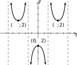
Figure 11.164 Asymptotes: , , , …
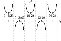
Figure 11.165
In Exercises -, the graph of a (co)tangent function given. Find a formula the function in the form and . Select so . Check your answer by graphing.
Asymptotes: , , , …
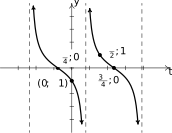
Figure 11.166 Asymptotes: , , , …
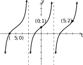
Figure 11.167
In Section 11.3.2, we observed9 that the cosine and sine functions are continuous. As such, the other four circular functions are continuous on their domains.10
In Exercises -, determine the given limit. Use the symbols `' and `'as appropriate. Check your answers graphically.
- .
- .
In Exercise in Section 11.4, we proved .
- Use Theorem 6.2 from Section 6.1 to show .
- Which indeterminate form is present in the limit ?
- Graph near . What appears to be the limit?
- Rewrite in terms of and and use part to analytically find .
- Use the same methodology as above to help you analytically determine
- Use the conversion formulas listed in Theorem 11.5 to create conversion formulas between secant and cosecant functions.
- Use a conversion formula to rewrite our first answer to Example 11.5.2, , in terms of cosecants.
- Rework Example 11.5.2 and find answers with .
- Prove Theorem 11.11 using Theorem 11.6.
- Prove Theorem 11.13 using Theorem 5.11.
In this Exercise, we argue the range of the tangent function is . Let be a fixed, but arbitrary positive real number.
- Show there is an acute angle with . (Hint: think right triangles.)
- Using the symmetry of the Unit Circle, explain why there are angles with .
- Find angles with .
- Combine the three parts above to conclude the range of the tangent function is .
- Prove is odd. (Hint: mimic the proof given in the text that is odd.)
Answers
Period:
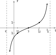
Figure 11.168 Period:
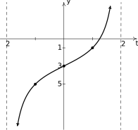
Figure 11.169 is equivalent to via the Even / Odd identity for tangent. Period:
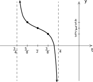
Figure 11.170 Start with Period:
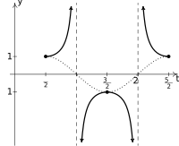
Figure 11.171 Start with Period:
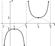
Figure 11.172 Start with Period:
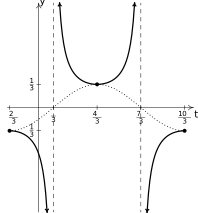
Figure 11.173 Start with Period:
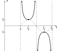
Figure 11.174 Start with Period:
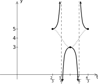
Figure 11.175 Start with Period:
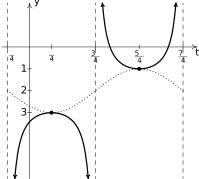
Figure 11.176 Period:
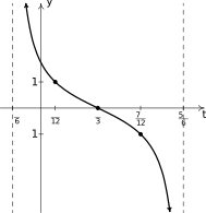
Figure 11.177 Period:
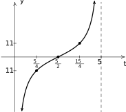
Figure 11.178 Period:
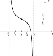
Figure 11.179 - ,
- ,
- ,
- ,
- .
- .
- As , .
- The graph of approaches so appears to be .
- .
- and .
- , in terms of cosecants.
- and are two answers
Adapted from Precalculus with Integrated Calculus, edition 4i, by Carl Stitz and Jeff Zeager (stitz-zeager.com), licensed under CC BY-NC-SA 3.0. Changes were made: reformatted as an accessible XYZ web edition. License: CC-BY-NC-SA-3.0.