11.3 Graphs of Sine and Cosine

On page Section 11.2, we discussed how to interpret the sine and cosine of real numbers. To review, we identify a real number $t$ with an oriented angle $θ$ measuring $t$ radians¹ and define $\sin (t) = \sin (θ)$ and $\cos (t) = \cos (θ)$ . Since every real number can be identified with one and only one angle $θ$ this way, the domains of the functions $f (t) = \sin (t)$ and $g (t) = \cos (t)$ are all real numbers, $open parenthesis minus ∞, ∞ close parenthesis$ .

When it comes to range, recall that the sine and cosine of angles are coordinates of points on the Unit Circle and hence, each fall between $minus 1$ and $1$ inclusive. Since the real number line,² when wrapped around the Unit Circle completely covers the circle, we can be assured that every point on the Unit Circle corresponds to at least one real number. Putting these two facts together, we conclude the range of $f (t) = \sin (t)$ and $g (t) = \cos (t)$ are both $open bracket minus 1, 1 close bracket$ . We summarize these two important facts below.

Theorem

Domain and Range of the Cosine and Sine Functions:

Table 11.1

∙

The function

f (t) = \sin (t)

∙

The function

g (t) = \cos (t)

[4pt] – has domain

open parenthesis minus ∞, ∞ close parenthesis

– has domain

open parenthesis minus ∞, ∞ close parenthesis

[4pt] – has range

open bracket minus 1, 1 close bracket

– has range

open bracket minus 1, 1 close bracket

[4pt]

Our aim in this section is to become familiar with the graphs of $f (t) = \sin (t)$ and $g (t) = \cos (t)$ . To that end, we begin by making a table and plotting points. We'll start by graphing $f (t) = \sin (t)$ by making a table of values and plotting the corresponding points. We'll keep the independent variable ` $t$ ' for now and use the default ` $y$ ' as our dependent variable.³ Note in the graph below, on the right, the scale of the horizontal and vertical axis is far from 1:1. (We will present a more accurately scaled graph shortly.)

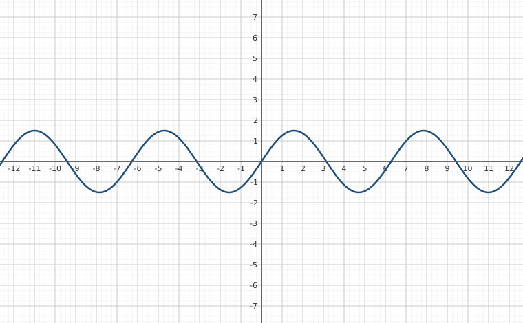
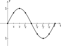
$\begin{matrix} t & \sin (t) & (t, \sin (t)) \\ 0 & 0 & (0, 0) \\ \frac{π}{4} & \frac{\sqrt{2}}{2} & (\frac{π}{4}, \frac{\sqrt{2}}{2}) \\ \frac{π}{2} & 1 & (\frac{π}{2}, 1) \\ \frac{3 π}{4} & \frac{\sqrt{2}}{2} & (\frac{3 π}{4}, \frac{\sqrt{2}}{2}) \\ π & 0 & (π, 0) \\ \frac{5 π}{4} & - \frac{\sqrt{2}}{2} & (\frac{5 π}{4}, - \frac{\sqrt{2}}{2}) \\ \frac{3 π}{2} & - 1 & (\frac{3 π}{2}, - 1) \\ \frac{7 π}{4} & - \frac{\sqrt{2}}{2} & (\frac{7 π}{4}, - \frac{\sqrt{2}}{2}) \\ 2 π & 0 & (2 π, 0) \end{matrix}$

Figure: Graphing . — **Figure 11.84** Graphing $y = \sin (t)$ .

If we plot additional points, we soon find that the graph repeats itself. This shouldn't come as too much of a surprise considering Theorem 11.2. In fact, in light of that theorem, we expect the function to repeat itself every $2 ⁢ π$ units. Below is a more accurately scaled graph highlighting the portion we had already graphed above. The graph is often described as having a `wavelike' nature and is sometimes called a sine wave or, more technically, a sinusoid.

Figure: A more accurately scaled graph of . — **Figure 11.85** A more accurately scaled graph of $f (t) = \sin (t)$ .

Note that by copying the highlighted portion of the graph and pasting it end-to-end, we obtain the entire graph of $f (t) = \sin (t)$ . We give this `repeating' property a name.

Definition

Periodic Functions: A function $f$ is said to be periodic if there is a real number $c$ so that $f (t + c) = f (t)$ for all real numbers $t$ in the domain of $f$ . The smallest positive number $p$ for which $f (t + p) = f (t)$ for all real numbers $t$ in the domain of $f$ , if it exists, is called the period of $f$ .

We have already seen a family of periodic functions in Section 1.2: the constant functions. However, despite being periodic a constant function has no period. (We'll leave that odd gem as an exercise for you.)

Returning to $f (t) = \sin (t)$ , we see that by Definition 11.3, $f$ is periodic since $\sin (t + 2 π) = \sin (t)$ . To determine the period of $f$ , we need to find the smallest real number $p$ so that $f (t + p) = f (t)$ for all real numbers $t$ or, said differently, the smallest positive real number $p$ such that $\sin (t + p) = \sin (t)$ for all real numbers $t$ .

We know that $\sin (t + 2 π) = \sin (t)$ for all real numbers $t$ but the question remains if any smaller real number will do the trick. Suppose $p greater than 0$ and $\sin (t + p) = \sin (t)$ for all real numbers $t$ . Then, in particular, $\sin (0 + p) = \sin (0) = 0$ so that $sin ⁡ open parenthesis p close parenthesis equals 0$ . From this we know $p$ is a multiple of $π$ . Since $\sin (\frac{π}{2}) \neq \sin (\frac{π}{2} + π)$ , we know $p \neq π$ . Hence, $p equals 2 ⁢ π$ so the period of $f (t) = \sin (t)$ is $2 ⁢ π$ .

Having period $2 ⁢ π$ essentially means that we can completely understand everything about the function $f (t) = \sin (t)$ by studying one interval of length $2 ⁢ π$ , say $open bracket 0, 2 ⁢ π close bracket$ .⁴ In some advanced texts, the interval of choice is $[- π, π)$ . For this reason, when graphing sine (and cosine) functions, we typically restrict our attention to graphing these functions over the course of one period to produce one cycle of the graph.

Not surprisingly, the graph of $g (t) = \cos (t)$ exhibits similar behavior as $f (t) = \sin (t)$ as seen below.⁵

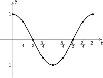
$\begin{matrix} t & \cos (t) & (t, \cos (t)) \\ 0 & 1 & (0, 1) \\ \frac{π}{4} & \frac{\sqrt{2}}{2} & (\frac{π}{4}, \frac{\sqrt{2}}{2}) \\ \frac{π}{2} & 0 & (\frac{π}{2}, 0) \\ \frac{3 π}{4} & - \frac{\sqrt{2}}{2} & (\frac{3 π}{4}, - \frac{\sqrt{2}}{2}) \\ π & - 1 & (π, - 1) \\ \frac{5 π}{4} & - \frac{\sqrt{2}}{2} & (\frac{5 π}{4}, - \frac{\sqrt{2}}{2}) \\ \frac{3 π}{2} & 0 & (\frac{3 π}{2}, 0) \\ \frac{7 π}{4} & \frac{\sqrt{2}}{2} & (\frac{7 π}{4}, \frac{\sqrt{2}}{2}) \\ 2 π & 1 & (2 π, 1) \end{matrix}$

Like $f (t) = \sin (t)$ , $g (t) = \cos (t)$ is a wavelike curve with period $2 ⁢ π$ . Moreover, the graphs of the sine and cosine functions have the same shape - differing only in what appears to be a horizontal shift. As we'll prove in Section 12.2, $\sin (t + \frac{π}{2}) = \cos (t)$ , which means we can obtain the graph of $y = \cos (t)$ by shifting the graph of $y = \sin (t)$ to the left $\frac{π}{2}$ units.⁶

Figure: The graph of . — **Figure 11.87** The graph of $g (t) = \cos (t)$ .

While arguably the most important property shared by $f (t) = \sin (t)$ and $g (t) = \cos (t)$ is their periodic `wavelike' nature,⁷ their graphs suggest these functions are both continuous and smooth. Recall from Section 2.1 that, like polynomial functions, the graphs of the sine and cosine functions have no jumps, gaps, holes in the graph, vertical asymptotes, corners or cusps.

Note the graphs of both $f (t) = \sin (t)$ and $g (t) = \cos (t)$ meander as $t → minus ∞$ or as $→ ∞$ . Said differently, none of the limits $lim t → minus ∞ sin ⁡ open parenthesis t close parenthesis$ , $lim t → ∞ sin ⁡ open parenthesis t close parenthesis$ , $lim t → minus ∞ cos ⁡ open parenthesis t close parenthesis$ , or $lim t → ∞ cos ⁡ open parenthesis t close parenthesis$ exist. Even though these functions are `trapped' (or bounded) between $minus 1$ and $1$ , neither graph has any horizontal asymptotes.

Lastly, the graphs of $f (t) = \sin (t)$ and $g (t) = \cos (t)$ suggest each enjoy one of the symmetries introduced in Section 2.1. The graph of $y = \sin (t)$ appears to be symmetric about the origin while the graph of $y = \cos (t)$ appears to be symmetric about the $y$ -axis. Indeed, as we'll prove in Section 12.2, $f (t) = \sin (t)$ is, in fact, an odd function: ⁸ that is, $\sin (- t) = - \sin (t)$ and $g (t) = \cos (t)$ is an even function, so $\cos (- t) = \cos (t)$ .

We summarize all of these properties in the following result.

Theorem

Properties of the Cosine and Sine Functions

Table 11.2

∙

The function

f (t) = \sin (t)

∙

The function

g (t) = \cos (t)

– has domain

open parenthesis minus ∞, ∞ close parenthesis

– has domain

open parenthesis minus ∞, ∞ close parenthesis

[4pt] – has range

open bracket minus 1, 1 close bracket

– has range

open bracket minus 1, 1 close bracket

[4pt] – is continuous and smooth

– is continuous and smooth

[4pt] – is odd

– is even

[4pt] – has period

2 ⁢ π

– has period

2 ⁢ π

$∙$ Conversion formulas: $\sin (t + \frac{π}{2}) = \cos (t)$ and $\cos (t - \frac{π}{2}) = \sin (t)$

Now that we know the basic shapes of the graphs of $y = \sin (t)$ and $y = \cos (t)$ , we can use the results of Section 5.4 to graph more complicated functions using transformations. The fact that both of these functions are periodic means we only have to know what happens over the course of one period of the function in order to determine what happens to all points on the graph. To that end, we graph the `fundamental cycle' - the portion of each graph generated over the interval $open bracket 0, 2 ⁢ π close bracket$ - for each sine and cosine:

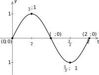
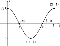
Figure: The `fundamental cycle' of . — **Figure 11.88** The `fundamental cycle' of $y = \sin (t)$ .

In working through Section 5.4, it was very helpful to track `key points' through the transformations. The `key points' we've indicated on the graphs above correspond to the quadrantal angles and generate the zeros and the extrema of functions. Since the quadrantal angles divide the interval $open bracket 0, 2 ⁢ π close bracket$ into four equal pieces, we shall refer to these angles henceforth as the `quarter marks.'

It is worth noting that because the transformations discussed in Section 5.4 are linear,⁹ the relative spacing of the points before and after the transformations remains the same.¹⁰ In particular, wherever the interval $open bracket 0, 2 ⁢ π close bracket$ is mapped, the quarter marks of the new interval correspond to the quarter marks of $open bracket 0, 2 ⁢ π close bracket$ . (Can you see why?) We will exploit this fact in the following example.

Example 1

Graph one cycle of the following functions. State the period of each.

$f ⁢ open parenthesis t close parenthesis equals 3 ⁢ sin ⁡ open parenthesis 2 ⁢ t close parenthesis$
$g (t) = 2 \cos (t + \frac{π}{2}) + 1$

One way to proceed is to use Theorem 5.11 and follow the procedure outlined there. Starting with the fundamental cycle of $y = \sin (t)$ , we divide each $t$ -coordinate by $2$ and multiply each $y$ -coordinate by 3 to obtain one cycle of $y equals 3 ⁢ sin ⁡ open parenthesis 2 ⁢ t close parenthesis$ .
Figure 11.90 The `fundamental cycle' of $y = \sin (t)$ .
Figure 11.91 One cycle of $y equals 3 ⁢ sin ⁡ open parenthesis 2 ⁢ t close parenthesis$ .
Since one cycle of $y = f (t)$ is completed over the interval $open bracket 0, π close bracket$ , the period of $f$ is $π$ .
Starting with the fundamental cycle of $y = \cos (t)$ and using Theorem 5.11, we subtract $\frac{π}{2}$ from each of the $t$ -coordinates, then multiply each $y$ -coordinate by $2$ , and add $1$ to each $y$ -coordinate.
We find one cycle of $y = g (t)$ is completed over the interval $[- \frac{π}{2}, \frac{3 π}{2}]$ , the period is $\frac{3 π}{2} - (- \frac{π}{2}) = 2 π$ .
Figure 11.92 The `fundamental cycle' of $y = \cos (t)$ .
Figure 11.93 One cycle of $y = 2 \cos (t + \frac{π}{2})$ +1

As previously mentioned, the curves graphed in Example 11.3.1 are examples of sinusoids. A sinusoid is the result of taking the graph of $y = \sin (t)$ or $y = \cos (t)$ and performing any of the transformations mentioned in Section 5.4. We graph one cycle of a generic sinusoid below. Sinusoids can be characterized by four properties: period, phase shift, vertical shift (or `baseline'), and amplitude.

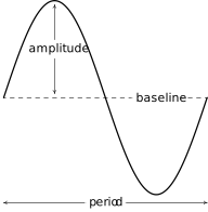
Coordinate-plane figure. — **Figure 11.94**

We have already discussed the period of a sinusoid. If we think of $t$ as measuring time, the period is how long it takes for the sinusoid to complete one cycle and is usually represented by the letter $T$ . The standard period of both $\sin (t)$ and $\cos (t)$ is $2 ⁢ π$ , but horizontal scalings will change this.

In Example 11.3.1, for instance, the function $f ⁢ open parenthesis t close parenthesis equals 3 ⁢ sin ⁡ open parenthesis 2 ⁢ t close parenthesis$ has period $π$ instead of $2 ⁢ π$ because the graph is horizontally compressed by a factor of $2$ as compared to the graph of $y = \sin (t)$ . However, the period of $g (t) = 2 \cos (t + \frac{π}{2}) + 1$ is the same as the period of $\cos (t)$ , $2 ⁢ π$ , since there are no horizontal scalings.

The phase shift of the sinusoid is the horizontal shift. Again, thinking of $t$ as time, the phase shift of a sinusoid can be thought of as when the sinusoid `starts' as compared to $t equals 0$ . Assuming there are no reflections across the $y$ -axis, we can determine the phase shift of a sinusoid by finding where the value $t equals 0$ on the graph of $y = \sin (t)$ or $y = \cos (t)$ is mapped to under the transformations.

For $f ⁢ open parenthesis t close parenthesis equals 3 ⁢ sin ⁡ open parenthesis 2 ⁢ t close parenthesis$ , the phase shift is ` $0$ ' since the value $t equals 0$ on the graph of $y = \sin (t)$ remains stationary under the transformations. Loosely speaking, this means both $y = \sin (t)$ and $y equals 3 ⁢ sin ⁡ open parenthesis 2 ⁢ t close parenthesis$ `start' at the same time. The phase shift of $g (t) = 2 \cos (t + \frac{π}{2}) + 1$ is $- \frac{π}{2}$ or ` $\frac{π}{2}$ to the left' since the value $t equals 0$ on the graph of $y = \cos (t)$ is mapped to $t = - \frac{π}{2}$ on the graph of $y = 2 \cos (t + \frac{π}{2}) + 1$ . Again, loosely speaking, this means $y = 2 \cos (t + \frac{π}{2}) + 1$ starts $\frac{π}{2}$ time units earlier than $y = \cos (t)$ .

The vertical shift of a sinusoid is exactly the same as the vertical shifts in Section 5.4 and determines the new `baseline' of the sinusoid. Thanks to symmetry, the vertical shift can always be found by averaging the maximum and minimum values of the sinusoid. For $f ⁢ open parenthesis t close parenthesis equals 3 ⁢ sin ⁡ open parenthesis 2 ⁢ t close parenthesis$ , the vertical shift is $0$ whereas the vertical shift of $g (t) = 2 \cos (t + \frac{π}{2}) + 1$ is $1$ or ` $1$ up.'

The amplitude of the sinusoid is a measure of how `tall' the wave is, as indicated in the figure below. Said differently, the amplitude measures how much the curve gets displaced from its `baseline. ' The amplitude of the standard cosine and sine functions is $1$ , but vertical scalings can alter this.

In Example 11.3.1, the amplitude of $f ⁢ open parenthesis t close parenthesis equals 3 ⁢ sin ⁡ open parenthesis 2 ⁢ t close parenthesis$ is $3$ , owing to the vertical stretch by a factor of $3$ as compared with the graph of $y = \sin (t)$ . In the case of $g (t) = 2 \cos (t + \frac{π}{2}) + 1$ , the amplitude is $2$ due to its vertical stretch as compared with the graph of $y = \cos (t)$ . Note that the ` $plus 1$ ' here does not affect the amplitude of the curve; it merely changes the `baseline' from $y equals 0$ to $y equals 1$ .

The following theorem shows how these four fundamental quantities relate to the parameters which describe a generic sinusoid. The proof follows from Theorem 5.11 and is left to the reader in Exercise.

Theorem

For $ω greater than 0$ , the graphs of

$S (t) = A \sin (ω t + ϕ) + B and C (t) = A \cos (ω t + ϕ) + B$

have period $T = \frac{2 π}{ω}$
have amplitude $| A |$
have phase shift $- \frac{ϕ}{ω}$
have vertical shift or `baseline' $B$

The parameter $ω$ mentioned above is called the angular frequency, or more simply, the frequency of the sinusoid and is the number of cycles the sinusoid completes over an interval of length $2 ⁢ π$ . That is, $ω$ measures how `frequently' the sinusoid repeats over an interval of length $2 ⁢ π$ . As we'll see in the next example, we can always ensure $ω greater than 0$ using the even and odd properties of the cosine and sine functions, respectively. If $t$ represents time, $ω$ as represents how fast the sinusoid is being generated in terms of radians per unit time. In essence, it is the angular speed of the curve.

A quantity closely related to the angular frequency of the sinusoid is the ordinary frequency of the sinusoid, usually denoted $f$ . The ordinary frequency of a sinusoid measures the number of cycles the sinusoid completes over an interval of length $1$ . Since the period, $T$ represents the length of the interval required for a sinusoid to make one complete cycle, we have $f = \frac{1}{T}$ . Once again, if $t$ represents time, the ordinary frequency measures how fast the sinusoid is being generated in terms of complete cycles per unit time.¹¹

Note that since $T = \frac{2 π}{ω}$ , $f = \frac{1}{T} = \frac{ω}{2 π}$ . Rewriting, we get $ω equals 2 ⁢ π ⁢ f$ . To understand this equation in terms of units, recall $1$ complete cycle (revolution) around the Unit Circle counts for $2 ⁢ π$ radians. Hence, to get from $f$ , measured in cycles per unit time, to $ω$ , measured in radians per unit time, we need to multiply by $2 ⁢ π$ .

If the concepts of period and frequency seem familiar, they should. In Section 11.1, we discussed these very same ideas in the context of Example 11.1.3 and revisited them again in Section 11.2 in Equation 11.3. and Example 11.2.6. On the one hand, the notions presented here are more general, since they are not tied directly to circular motion. On the other hand, the stipulation in this section that $ω greater than 0$ means we are restricting our attention to angular speeds instead of the more general angular velocities.¹²

Last, but not least, the quantity $ϕ$ mentioned in Theorem 11.6 is called the phase or phase angle of the sinusoid. The phase of a sinusoid is the angle in the argument which corresponds to $t equals 0$ , and is important in describing waves in fields such as physics and electronics. When graphing sinusoids, however, we focus our attention on the horizontal shift induced by $ϕ$ , $- \frac{ϕ}{ω}$ .

We put Theorem 11.6 to good use in the next example.

Example 2

Use Theorem 11.6 to determine the frequency, period, phase shift, amplitude, and vertical shift of each of the following functions and use this information to graph one cycle of each function.

$f (t) = 3 \cos (\frac{π t - π}{2}) + 1$
$g (t) = \frac{1}{2} \sin (π - 2 t) + \frac{3}{2}$

To use Theorem 11.6, we first need to rewrite $f (t)$ in the form prescribed by Theorem 11.6. To that end, we rewrite: $f (t) = 3 \cos (\frac{π t - π}{2}) + 1 = 3 \cos (\frac{π}{2} t + (- \frac{π}{2})) + 1$ .
From this, we identify $A equals 3$ , $ω = \frac{π}{2}$ , $ϕ = - \frac{π}{2}$ and $B equals 1$ . According to Theorem 11.6, the frequency is $ω = \frac{π}{2}$ , the period is $T = \frac{2 π}{ω} = \frac{2 π}{π / 2} = 4$ , the phase shift is $- \frac{ϕ}{ω} = - \frac{- π / 2}{π / 2} = 1$ (indicating a shift to the right $1$ unit), the amplitude is $| A | = | 3 | = 3$ , and the vertical shift is $B equals 1$ (indicating a shift up $1$ unit.)
To graph $y = f (t)$ , we know one cycle begins at $t equals 1$ (the phase shift.) Since the period is $4$ , we know the cycle ends $4$ units later at $t = 1 + 4 = 5$ . If we divide the interval $open bracket 1, 5 close bracket$ into four equal pieces, each piece has length $\frac{4}{4} = 1$ . Hence, we to get our quarter marks, we start with $t equals 1$ and add $1$ unit until we reach the endpoint, $t equals 5$ . Our new quarter marks are: $t equals 1$ , $t equals 2$ , $t equals 3$ , $t equals 4$ , and $t equals 5$ .
We now substitute these new quarter marks into $f (t)$ to obtain the corresponding $y$ -values on the graph.¹³ We connect the dots in a `wavelike' fashion to produce the graph below on the right.
Note that we can (partially) spot-check our answer by noting the average of the maximum and minimum is $\frac{4 + (- 2)}{2} = 1$ (our vertical shift) and the amplitude, $4 - 1 = 1 - (- 2) = 3$ is indeed $3$ .
$\begin{matrix} t & f (t) & (t, f (t)) \\ 1 & 4 & (1, 4) \\ 2 & 1 & (2, 1) \\ 3 & - 2 & (3, - 2) \\ 4 & 1 & (4, 1) \\ 5 & 4 & (5, 4) \end{matrix}$
Figure 11.95 One cycle of $y = f (t)$ .
Thought not asked for, this example provides a nice opportunity to interpret the ordinary frequency: $f = \frac{1}{T} = \frac{1}{4}$ . Hence, $\frac{1}{4}$ of the sinusoid is traced out over an interval that is $1$ unit long.
Turning our attention now to the function $g$ , we first note that the coefficient of $t$ is negative. In order to use Theorem 11.6, we need that coefficient to be positive. Hence, we first use the odd property of the sine function to rewrite $sin ⁡ open parenthesis π minus 2 ⁢ t close parenthesis$ so that instead of a coefficient of $minus 2$ , $t$ has a coefficient of $2$ . We get $\sin (π - 2 t) = \sin (- 2 t + π) = \sin (- (2 t - π)) = - \sin (2 t - π)$ . Hence, $g (t) = - \frac{1}{2} \sin (2 t + (- π)) + \frac{3}{2}$ .
We idenitfy $A = - \frac{1}{2}$ , $ω equals 2$ , $ϕ = - π$ and $B = \frac{3}{2}$ . The frequency is $ω equals 2$ , the period is $T = \frac{2 π}{2} = π$ , the phase shift is $- \frac{- π}{2} = \frac{π}{2}$ (indicating a shift right $\frac{π}{2}$ units), the amplitude is $| - \frac{1}{2} | = \frac{1}{2}$ , and, finally, the vertical shift is up $\frac{3}{2}$ .
Proceeding as before, we know one cycle of $g$ starts at $t = \frac{π}{2}$ and ends at $t = \frac{π}{2} + π = \frac{3 π}{2}$ . Dividing the interval $[\frac{π}{2}, \frac{3 π}{2}]$ into four equal pieces gives pieces of length $\frac{π}{4}$ units. Hence, to obtain our new quarter marks, we start at $t = \frac{π}{2}$ and add $\frac{π}{4}$ until we reach $t = \frac{3 π}{2}$ . Our new quarter marks are: $t = \frac{π}{2}$ , $t = \frac{3 π}{4}$ , $t = π$ , $t = \frac{5 π}{4}$ , $t = \frac{3 π}{2}$ . Substituting these values into $g$ gives us the points to plot to produce the graph below on the right.
Again, we can quickly check the vertical shift by averaging the maximum and minimum values: $\frac{2 + 1}{2} = \frac{3}{2}$ and verify the amplitude: $2 - \frac{3}{2} = \frac{3}{2} - 1 = \frac{1}{2}$ .
$\begin{matrix} t & g (t) & (t, g (t)) \\ \frac{π}{2} & \frac{3}{2} & (\frac{π}{2}, \frac{3}{2}) \\ \frac{3 π}{4} & 1 & (\frac{3 π}{4}, 1) \\ π & \frac{3}{2} & (π, \frac{3}{2}) \\ \frac{5 π}{4} & 2 & (\frac{5 π}{4}, 2) \\ \frac{3 π}{2} & \frac{3}{2} & (\frac{3 π}{2}, \frac{3}{2}) \end{matrix}$
Figure 11.96 One cycle of $y = g (t)$ .

Note that in this section, we have discussed two ways to graph sinusoids: using Theorem 5.11 from Section 5.4 and using Theorem 11.6. Both methods will produce one cycle of the resulting sinusoid, but each method may produce a different cycle of the same sinusoid.

For example, if we graphed the function $g (t) = \frac{1}{2} \sin (π - 2 t) + \frac{3}{2}$ from Example 11.3.2 using Theorem 5.11, we obtain the following:

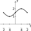
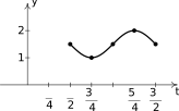
$\begin{matrix} t & g (t) & (t, g (t)) \\ \frac{π}{2} & \frac{3}{2} & (\frac{π}{2}, \frac{3}{2}) \\ \frac{π}{4} & 2 & (\frac{π}{4}, 2) \\ 0 & \frac{3}{2} & (0, \frac{3}{2}) \\ - \frac{π}{4} & 1 & (- \frac{π}{4}, 1) \\ - \frac{π}{2} & \frac{3}{2} & (- \frac{π}{2}, \frac{3}{2}) \end{matrix}$

Figure: One cycle via Theorem . — **Figure 11.97** One cycle via Theorem 5.11.

Comparing this result with the one obtained in Example 11.3.2 side by side, we see that one cycle ends right where the other starts. The cause of this discrepancy goes back to using the odd property of sine.

Essentially, the odd property of the sine function converts a reflection across the $y$ -axis into a reflection across the $t$ -axis. (Can you see why?) For this reason, whenever the coefficient of $t$ is negative, Theorems 5.11 and 11.6 will produce different results.

In the Exercises, we assume the problems are worked using Theorem 11.6. If you choose to use Theorems 5.11 instead, your answer may look different than what is provided even though both your answer and the textbook's answer represent one cycle of the same function.

In the next example, we use Theorem 11.6 to determine the formula of a sinusoid given the graph of one cycle. Note that in some disciplines, sinusoids are written in terms of sines whereas in others, cosines functions are preferred. To cover all bases, we ask for both.

Example 3

Below is the graph of one complete cycle of a sinusoid $y = f (t)$ .

Figure 11.99 One cycle of

y = f (t)

Write $f (t)$ in the form $C (t) = A \cos (ω t + ϕ) + B$ , for $ω greater than 0$ .
Write $f (t)$ in the form $S (t) = A \sin (ω t + ϕ) + B$ , for $ω greater than 0$ .

Since one cycle is graphed over the interval $open bracket minus 1, 5 close bracket$ , its period is $T = 5 - (- 1) = 6$ . According to Theorem 11.6, $6 = T = \frac{2 π}{ω}$ , so that $ω = \frac{π}{3}$ . Next, we see that the phase shift is $minus 1$ , so we have $- \frac{ϕ}{ω} = - 1$ , or $ϕ = ω = \frac{π}{3}$ .
To find the baseline, we average the maximum and minimum values: $B = \frac{1}{2} [\frac{5}{2} + (- \frac{3}{2})] = \frac{1}{2} (1) = \frac{1}{2}$ . To find the amplitude, we subtract the maximum value from the baseline: $A = \frac{5}{2} - \frac{1}{2} = 2$ .
Putting this altogether, we obtain our final answer is $f (t) = 2 \cos (\frac{π}{3} t + \frac{π}{3}) + \frac{1}{2}$ .
Since we have written $f (t)$ in terms of cosines, we can use the conversion from sine to cosine as listed in Theorem 11.5. Since $\cos (t) = \sin (t + \frac{π}{2})$ , $\cos (\frac{π}{3} t + \frac{π}{3}) = \sin ([\frac{π}{3} t + \frac{π}{3}] + \frac{π}{2})$ , so $\cos (\frac{π}{3} t + \frac{π}{3}) = \sin (\frac{π}{3} t + \frac{5 π}{6})$ . Our final answer is $f (t) = 2 \sin (\frac{π}{3} t + \frac{5 π}{6}) + \frac{1}{2}$ .
However, for the sake of completeness, we provide another solution strategy which enables us to write $f (t)$ in terms of sines without starting with our answer from part 1.
Note that we obtain the period, amplitude, and vertical shift as before: $ω = \frac{π}{3}$ , $A equals 2$ and $B = \frac{1}{2}$ . The trickier part is finding the phase shift.
To that end, we imagine extending the graph of the given sinusoid as in the figure below so that we can identify a cycle beginning at $(\frac{7}{2}, \frac{1}{2})$ . Taking the phase shift to be $\frac{7}{2}$ , we get $- \frac{ϕ}{ω} = \frac{7}{2}$ , or $ϕ = - \frac{7}{2} ω = - \frac{7}{2} (\frac{π}{3}) = - \frac{7 π}{6}$ . Hence, our answer is $f (t) = 2 \sin (\frac{π}{3} t - \frac{7 π}{6}) + \frac{1}{2}$ .
Figure 11.100 Extending the graph of $y = f (t)$ .

Note that each of the answers given in Example 11.3.3 is one choice out of many possible answers. For example, when fitting a sine function to the data, we could have chosen to start at $(\frac{1}{2}, \frac{1}{2})$ taking $A = - 2$ . In this case, the phase shift is $\frac{1}{2}$ so $ϕ = - \frac{π}{6}$ for an answer of $f (t) = - 2 \sin (\frac{π}{3} t - \frac{π}{6}) + \frac{1}{2}$ . The ultimate check of any solution is to graph the answer and check it matches the given data.

Applications of Sinusoids

In the same way exponential functions can be used to model a wide variety of phenomena in nature,¹⁴ the sine and cosine functions can be used to model their fair share of natural behaviors. Our first foray into sinusoidal motion revisits circular motion - in particular Equation 11.3.

Example 4

Recall from Exercise in Section 11.1 that The Giant Wheel at Cedar Point is a circle with diameter 128 feet which sits on an 8 foot tall platform making its overall height 136 feet. It completes two revolutions in 2 minutes and 7 seconds. Assuming that the riders are at the edge of the circle, find a sinusoid which describes the height of the passengers above the ground $t$ seconds after they pass the point on the wheel closest to the ground.

We sketch the problem situation below and assume a counter-clockwise rotation.¹⁵

Figure 11.101

We know from the equations given on page 11.3 in Section 11.2.1 that the $y$ -coordinate for counter-clockwise motion on a circle of radius $r$ centered at the origin with constant angular velocity (frequency) $ω$ is given by $y = r \sin (ω t)$ . Here, $t equals 0$ corresponds to the point $open parenthesis r, 0 close parenthesis$ so that $θ$ , the angle measuring the amount of rotation, is in standard position.

In our case, the diameter of the wheel is 128 feet, so the radius is $r equals 64$ feet. Since the wheel completes two revolutions in 2 minutes and 7 seconds (which is $127$ seconds) the period $T = \frac{1}{2} (127) = \frac{127}{2}$ seconds. Hence, the angular frequency is $ω = \frac{2 π}{T} = \frac{4 π}{127}$ radians per second.

Putting these two pieces of information together, we have that $y = 64 \sin (\frac{4 π}{127} t)$ describes the $y$ -coordinate on the Giant Wheel after $t$ seconds, assuming it is centered at $open parenthesis 0, 0 close parenthesis$ with $t equals 0$ corresponding to point $Q$ .

In order to find an expression for $h$ , we take the point $O$ in the figure as the origin. Since the base of the Giant Wheel ride is $8$ feet above the ground and the Giant Wheel itself has a radius of $64$ feet, its center is $72$ feet above the ground. To account for this vertical shift upward,¹⁶ we add $72$ to our formula for $y$ to obtain the new formula $h = y + 72 = 64 \sin (\frac{4 π}{127} t) + 72$ .

Next, we need to adjust things so that $t equals 0$ corresponds to the point $P$ instead of the point $Q$ . This is where the phase comes into play. Geometrically, we need to shift the angle $θ$ in the figure back $\frac{π}{2}$ radians.

From the discussion on page 11.3, we know $θ = ω t = \frac{4 π}{127} t$ , so we (temporarily) write the height in terms of $θ$ as $h = 64 \sin (θ) + 72$ . Subtracting $\frac{π}{2}$ from $θ$ gives $h (t) = 64 \sin (θ - \frac{π}{2}) + 72 = 64 \sin (\frac{4 π}{127} t - \frac{π}{2}) + 72$ .

We can check the reasonableness of our answer by graphing $y = h (t)$ over the interval $[0, \frac{127}{2}]$ and visualizing the path of a person on the Big Wheel ride over the course of one rotation.

Figure 11.102

A few remarks about Example 11.3.4 are in order. First, note that the amplitude of $64$ in our answer corresponds to the radius of the Giant Wheel. This means that passengers on the Giant Wheel never stray more than $64$ feet vertically from the center of the Wheel, which makes sense. Second, the phase shift of our answer works out to be $\frac{π / 2}{4 π / 127} = \frac{127}{8} = 15.875$ . This represents the `time delay' (in seconds) we introduce by starting the motion at the point $P$ as opposed to the point $Q$ . Said differently, passengers which `start' at $P$ take $15.875$ seconds to `catch up' to the point $Q$ .

Our next example revisits the daylight data first introduced in Section 1.4, Exercise.

Example 5

According to the U.S. Naval Observatory website, the number of hours $H$ of daylight that Fairbanks, Alaska received on the 21st day of the $n$ th month of 2009 is given below. Here $t equals 1$ represents January 21, 2009, $t equals 2$ represents February 21, 2009, and so on.

**Table 11.3**
Month
Number	1	2	3	4	5	6	7	8	9	10	11	12
Hours of
Daylight	5.8	9.3	12.4	15.9	19.4	21.8	19.4	15.6	12.4	9.1	5.6	3.3

Find a sinusoid which models these data and graph your answer along with the data.
Compare your answer to part to one obtained using the regression feature of a graphing utility.

To get a feel for the data, we plot it below on the left. At first glance, the data appear to be more like ` $∧$ '-shaped instead of sinusoidal, harkening back to Section 1.3. However, from experience, the hours of daylight is a cyclical process, which is why we attempt to fit this data to a sine function.
Please note that when it comes down to it, fitting a sinusoid to data manually is not an exact science. We do our best to find the constants $A$ , $ω$ , $ϕ$ and $B$ so that the function $H (t) = A \sin (ω t + ϕ) + B$ closely matches the data. In this example, we first go after the vertical shift $B$ to determine the baseline.
In a typical sinusoid, the value of $B$ is the average of the maximum and minimum values. So here we take $B = \frac{3.3 + 21.8}{2} = 12.55$ .
Next is the amplitude $A$ which is the displacement from the baseline to the maximum (and minimum) values. We find $A = 21.8 - 12.55 = 12.55 - 3.3 = 9.25$ . At this stage, our sinusoid has the form: $H (t) = 9.25 \sin (ω t + ϕ) + 12.55$ .
We proceed to find the angular frequency, $ω$ . Since the data collected is over the span of a year (12 months), we take the period $T equals 12$ months.¹⁷ This means $ω = \frac{2 π}{T} = \frac{2 π}{12} = \frac{π}{6}$ .
The last quantity to find is the phase $ϕ$ . Unlike the previous example, it is easier in this case to find the phase shift $- \frac{ϕ}{ω}$ . Since we picked $A greater than 0$ , the phase shift corresponds to the first value of $t$ with $H ⁢ open parenthesis t close parenthesis equals 12.55$ (the baseline value).¹⁸
Here, we choose $t equals 3$ , since its corresponding $H$ value of $12.4$ is closer to $12.55$ than the next value, $15.9$ , which corresponds to $t equals 4$ . Hence, $- \frac{ϕ}{ω} = 3$ , so $ϕ = - 3 ω = - 3 (\frac{π}{6}) = - \frac{π}{2}$ . We have $H (t) = 9.25 \sin (\frac{π}{6} t - \frac{π}{2}) + 12.55$ . Below on the right is a graph of our data with the curve $y = H (t)$ .
Figure 11.103
Figure 11.104
Plotting the data.
Plotting the data long with $y = H (t)$
Using desmos to find a regression model produces $A approximately equals 8.36$ and $B approximately equals 12.06$ , which closely match our answers from number. However, desmos calculates $ω \approx - 294.81$ and $ϕ \approx - 26.53$ , which are far from our values $ω = \frac{π}{6}$ and $ϕ = - \frac{π}{2}$ .
Indeed, in Exercise, we invite the reader to graph $y = 8.36 \sin (- 294.81 t - 26.53) + 12.06$ using desmos. At first glance, appears to be a solid gray rectangle. After zooming in, however, we see this rectangle is made up of literally hundreds of oscillations. Though desmos boasts this regression as having an $R^{2}$ value of $0.9886$ , meaning mathematically, this is a very good fit to the data, this curve doesn't model the real-world phenomenon of daylight hours in any sort of reasonable manner.
Since we know the period of the sinusoid is 12 months, we set $ω = \frac{π}{6}$ and ask desmos to run a regression for the remaining three parameters. Desmos returns the values $A \approx - 8.13$ , $B approximately equals 12.5$ , and $ϕ \approx - 4.70$ , with an $R^{2}$ value of $0.987$ , so its regression curve is a much more reasonable $H (t) = - 8.13 \sin (\frac{π}{6} t - 4.70) + 12.5$ . Even though, at first glance, this curve appears much different from our solution to number, the we graph both functions below on the right and see they are very similar.¹⁹ (Our solution to number is the darker of the two curves.)
Figure 11.105
Figure 11.106
Plotting the desmos's regression curve.
Plotting both solutions.

The scenario described in Example 11.3.5 is a typical example of where the circular functions are useful outside the context of angles or circular motion. Indeed, sine and cosine functions are used extensively to model a wide range of periodic phenomena including signal analysis, wave physics, and even quantum mechanics. We close this section discussing limits involving sine and cosine.

Limits involving Sine and Cosine

We've already stated as fact (but not proven) that $f (t) = \sin (t)$ and $g (t) = \cos (t)$ are continuous. Per Definition 6.4, this means that $lim_{t \to a} \sin (t) = \sin (a)$ and $lim_{t \to a} \cos (t) = \cos (a)$ for all real numbers, $a$ . This means, for instance, we can compute $lim_{t \to π} \cos (t) = \cos (π) = - 1$ . Per the discussion following Definition 6.4, so long as we avoid the usual domain pitfalls, we can also compute:

$lim_{t \to π} \frac{2 t \cos (t) - \sin (3 t)}{\sqrt{\cos (2 t)}} = \frac{2 π \cos (π) - \sin (3 π)}{\sqrt{\cos (2 π)}} = \frac{- 2 π - 0}{\sqrt{1}} = - 2 π$

In the next example we investigate a few (similar looking) limits of sinusoids.

Example 6

Investigate the following limits numerically, graphically, and analytically.

$lim t → 0$ $\sin (\frac{π}{t})$
$lim t → 0$ $sin ⁡ open parenthesis 10 to the power 23 ⁢ t close parenthesis$
$lim t → 0$ $\frac{\sin (t)}{t}$

To analyze $lim t → 0$ $\sin (\frac{π}{t})$ numerically, we construct a table of values `near' $t equals 0$ for $F (t) = \sin (\frac{π}{t})$ . Choosing values such as $t = \pm 0.001$ , $t = \pm 0.01$ , etc., we get a list of ` $0$ 's. This result shouldn't be too surprising since in each of these cases, $\frac{π}{t}$ results in an integer multiple of $π$ . However, the graph near $t equals 0$ (literally) paints a different picture. The graph appears to wildly oscillate near $t equals 0$ , suggesting that $lim t → 0$ $\sin (\frac{π}{t})$ does not exist.
Figure 11.107
Indeed, as $t \to 0^{-}$ , $\frac{π}{t} \to - \infty$ and as $t \to 0^{+}$ , $\frac{π}{t} \to \infty$ . In other words, all of the infinite oscillations experienced by the standard sine function, $f (t) = \sin (t)$ as $t → minus ∞$ and as $t → ∞$ are being brought back to near $t equals 0$ in $F (t) = \sin (\frac{π}{t})$ . Hence, $lim t → 0$ $\sin (\frac{π}{t})$ does not exist.
We proceed as above to investigate $lim t → 0$ $sin ⁡ open parenthesis 10 to the power 23 ⁢ t close parenthesis$ . A table and a graph of $F (t) = \sin (10^{23} t)$ `near' $t equals 0$ produces numerical and graphical noise. Neither the table nor the graph suggest $lim t → 0 F ⁢ open parenthesis t close parenthesis$ exists. However, we know $F (t) = \sin (10^{23} t)$ is a sinusoid with frequency $ω = 10^{23}$ . Zooming in by a factor of $10 to the power 23$ , we get one cycle of $F$ which suggests the limit is, in fact, $0$ .
Figure 11.108
Figure 11.109
$F (t) = \sin (10^{23} t)$ `near' $t equals 0$
$F (t) = \sin (10^{23} t)$ `nearer to ' $t equals 0$
Indeed, we know $F (t) = \sin (10^{23} t)$ is continuous, so $lim t → 0$ $\sin (10^{23} t) = \sin (10^{23} (0))) = \sin (0) = 0$ .
Next we investigate $F (t) = \frac{\sin (t)}{t}$ near $t equals 0$ . The table and graph both suggest $lim t → 0$ $\frac{\sin (t)}{t} = 1$ .
Figure 11.110
Attempting to analyze this limit analytically, we see that $lim t → 0$ $\frac{\sin (t)}{t}$ produces the indeterminate form ` $\frac{0}{0}$ '. At this stage, we do not have the tools to either prove or disprove our conjecture that $lim t → 0$ $\frac{\sin (t)}{t} = 1$ , but we will soon, ²⁰ so stay tuned!

Exercises

In Exercises -, graph one cycle of the given function. State the period, amplitude, phase shift and vertical shift of the function.

$f ⁢ open parenthesis t close parenthesis equals 3 ⁢ sin ⁡ open parenthesis t close parenthesis$
$g ⁢ open parenthesis t close parenthesis equals sin ⁡ open parenthesis 3 ⁢ t close parenthesis$
$h (t) = - 2 \cos (t)$
$f (t) = \cos (t - \frac{π}{2})$
$g (t) = - \sin (t + \frac{π}{3})$
$h (t) = \sin (2 t - π)$
$f (t) = - \frac{1}{3} \cos (\frac{1}{2} t + \frac{π}{3})$
$g (t) = \cos (3 t - 2 π) + 4$
$h (t) = \sin (- t - \frac{π}{4}) - 2$
$f (t) = \frac{2}{3} \cos (\frac{π}{2} - 4 t) + 1$
$g (t) = - \frac{3}{2} \cos (2 t + \frac{π}{3}) - \frac{1}{2}$
$h (t) = 4 \sin (- 2 π t + π)$

In Exercises -, a sinusoid is graphed. Find a formula for the sinusoid in the form $S (t) = A \sin (ω t + ϕ) + B$ and $C (t) = A \cos (ω t + ϕ) + B$ . Select $ω$ so $ω greater than 0$ . Check your answer by graphing.

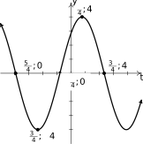
Figure 11.111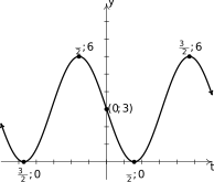
Figure 11.112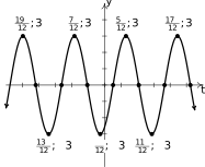
Figure 11.113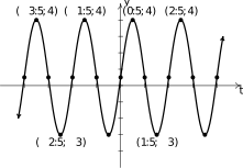
Figure 11.114
Use the graph of $S ⁢ open parenthesis t close parenthesis equals 4 ⁢ sin ⁡ open parenthesis t close parenthesis$ to graph each of the following functions. State the period of each.
1. $f ⁢ open parenthesis t close parenthesis equals vertical bar 4 ⁢ sin ⁡ open parenthesis t close parenthesis vertical bar$
2. $g (t) = \sqrt{4 \sin (t)}$

In Exercises -, use a graphing utility to help you and your classmates discuss the given questions.

Graph $f (t) = \cos (3 t) + \sin (t)$ . Is this function periodic? If so, what is the period?
Graph $f (t) = t \sin (t)$ along with $y = \pm t$ . What do you notice?
Graph $f (t) = \frac{\sin (t)}{t}$ along with $y = \pm \frac{1}{t}$ . What do you notice?
1. What appears to be $lim t → ∞ f ⁢ open parenthesis t close parenthesis$ ? Interpret your answer graphically.
2. Use the Squeeze Theorem, Theorem 10.2 from Section 10.1 to prove your claim.
  HINT: Since $minus 1 less than or equal to sin ⁡ open parenthesis t close parenthesis less than or equal to 1$ , for $t greater than 0$ , $- \frac{1}{t} \leq \frac{\sin (t)}{t} \leq \frac{1}{t}$ …
Graph $f (t) = \cos (\frac{1}{t})$ .
1. Investigate $lim t → 0 f ⁢ open parenthesis t close parenthesis$ . Does $lim t → 0 f ⁢ open parenthesis t close parenthesis$ exist? Why or why not?
2. Determine $lim t → ∞ f ⁢ open parenthesis t close parenthesis$ and interpret your answer graphically.
Graph $f (t) = e^{- 0.1 t} (\cos (2 t) + \sin (2 t))$ along with $y = \pm 2 e^{- 0.1 t}$ . What do you notice?
1. What appears to be $lim t → ∞ f ⁢ open parenthesis t close parenthesis$ ? Interpret your answer graphically.
2. Use the Squeeze Theorem, Theorem 10.2 from Section 10.1 to prove your claim.
  HINT: Since $minus 1 less than or equal to cos ⁡ open parenthesis 2 ⁢ t close parenthesis less than or equal to 1$ and $minus 1 less than or equal to sin ⁡ open parenthesis 2 ⁢ t close parenthesis less than or equal to 1$ , $- 2 \leq \cos (2 t) + \sin (2 t) \leq 2$ .
  Hence, $- 2 e^{- 0.1 t} \leq e^{- 0.1 t} (\cos (2 t) + \sin (2 t)) \leq 2 e^{- 0.1 t}$ …
Show every constant function $f$ is periodic by explaining why $f (x + 117) = f (x)$ for all real numbers $x$ . Then show that $f$ has no period by showing that you cannot find a smallest number $p$ such that $f (x + p) = f (x)$ for all real numbers $x$ .
Said differently, show that $f (x + p) = f (x)$ for all real numbers $x$ for ALL values of $p greater than 0$ , so no smallest value exists to satisfy the definition of `period'.
The sounds we hear are made up of mechanical waves. The note `A' above the note `middle C' is a sound wave with ordinary frequency $f equals 440$ Hertz $= 440 \frac{cycles}{second}$ . Find a sinusoid which models this note, assuming that the amplitude is $1$ and the phase shift is $0$ .
The voltage $V$ in an alternating current source has amplitude $220 ⁢ the square root of 2$ and ordinary frequency $f equals 60$ Hertz. Find a sinusoid which models this voltage. Assume that the phase is $0$ .
The London Eye is a popular tourist attraction in London, England and is one of the largest Ferris Wheels in the world. It has a diameter of 135 meters and makes one revolution (counter-clockwise) every 30 minutes. It is constructed so that the lowest part of the Eye reaches ground level, enabling passengers to simply walk on to, and off of, the ride. Find a sinsuoid which models the height $h$ of the passenger above the ground in meters $t$ minutes after they board the Eye at ground level.
On page 11.3 in Section 11.2.1, we found the $x$ -coordinate of counter-clockwise motion on a circle of radius $r$ with angular frequency $ω$ to be $x = r \cos (ω t)$ , where $t equals 0$ corresponds to the point $open parenthesis r, 0 close parenthesis$ . Suppose we are in the situation of Exercise above. Find a sinsusoid which models the horizontal displacement $x$ of the passenger from the center of the Eye in meters $t$ minutes after they board the Eye. Here we take $x ⁢ open parenthesis t close parenthesis greater than 0$ to mean the passenger is to the right of the center, while $x ⁢ open parenthesis t close parenthesis less than 0$ means the passenger is to the left of the center.
In Exercise in Section 11.1, we introduced the yo-yo trick `Around the World' in which a yo-yo is thrown so it sweeps out a vertical circle. As in that exercise, suppose the yo-yo string is 28 inches and it completes one revolution in 3 seconds. If the closest the yo-yo ever gets to the ground is 2 inches, find a sinsuoid which models the height $h$ of the yo-yo above the ground in inches $t$ seconds after it leaves its lowest point.
Consider the pendulum below. Ignoring air resistance, the angular displacement of the pendulum from the vertical position, $θ$ , can be modeled as a sinusoid.²¹
Figure 11.115
The amplitude of the sinusoid is the same as the initial angular displacement, $θ sub 0$ , of the pendulum and the period of the motion is given by
$T = 2 π \sqrt{\frac{ℓ}{g}}$
where $ℓ$ is the length of the pendulum and $g$ is the acceleration due to gravity.
1. Find a sinusoid which gives the angular displacement $θ$ as a function of time, $t$ . Arrange things so $θ ⁢ open parenthesis 0 close parenthesis equals θ sub 0$ .
2. In Exercise section 4.1, you found the length of the pendulum needed in Jeff's antique Seth-Thomas clock to ensure the period of the pendulum is $\frac{1}{2}$ of a second. Assuming the initial displacement of the pendulum is $15 degrees$ , find a sinusoid which models the displacement of the pendulum $θ$ as a function of time, $t$ , in seconds.

The table below lists the average temperature of Lake Erie as measured in Cleveland, Ohio on the first of the month for each month during the years 1971 – 2000.²² For example, $t equals 3$ represents the average of the temperatures recorded for Lake Erie on every March 1 for the years 1971 – 2000.

**Table 11.4**
Month
Number, $t$	1	2	3	4	5	6	7	8	9	10	11	12
Temperature
( $∘$ F), $T$	36	33	34	38	47	57	67	74	73	67	56	46

Using the techniques discussed in Example 11.3.5, fit a sinusoid to these data.
Graph your model along with the data set to judge the reasonableness of the fit.
Use the model from to predict the average temperature recorded for Lake Erie on April $15 to the power th$ and September $15 to the power th$ during the years 1971–2000.²³
Compare your results to those obtained using a graphing utility.

The fraction of the moon illuminated at midnight Eastern Standard Time on the $t^{th}$ day of June, 2009 is given in the table below.²⁴

**Table 11.5**
Day of
June, $t$	3	6	9	12	15	18	21	24	27	30
Fraction
Illuminated, $F$	0.81	0.98	0.98	0.83	0.57	0.27	0.04	0.03	0.26	0.58

Using the techniques discussed in Example 11.3.5, fit a sinusoid to these data.²⁵
Graph your model along with the data set to judge the reasonableness of the fit.
Use the model from to predict the fraction of the moon illuminated on June 1, 2009. ²⁶
Compare your results to those obtained using a graphing utility.

Use a graphing utility to graph $y = 8.36 \sin (- 294.81 t - 26.53) + 12.06$ . (This is the regression model produced by desmos in Example 11.3.5.) Zoom in, as needed, until you start to see the wave-like nature of the graph. Use Theorem 11.6 to determine a window which produces exactly one complete cycle of this sinusoid and check your answer graphically.
Use Theorem 5.11 to prove Theorem 11.6.
With the help of your classmates, research Amplitude Modulation and Frequency Modulation .
What other things in the world might be roughly sinusoidal? Look to see what models you can find for them and share your results with your class.

Answers

$f ⁢ open parenthesis t close parenthesis equals 3 ⁢ sin ⁡ open parenthesis t close parenthesis$ Period: $2 ⁢ π$ Amplitude: $3$ Phase Shift: $0$ Vertical Shift: $0$
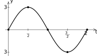
Figure 11.116
$g ⁢ open parenthesis t close parenthesis equals sin ⁡ open parenthesis 3 ⁢ t close parenthesis$ Period: $\frac{2 π}{3}$ Amplitude: $1$ Phase Shift: $0$ Vertical Shift: $0$
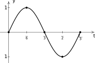
Figure 11.117
$h (t) = - 2 \cos (t)$ Period: $2 ⁢ π$ Amplitude: $2$ Phase Shift: $0$ Vertical Shift: $0$
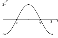
Figure 11.118
$f (t) = \cos (t - \frac{π}{2})$ Period: $2 ⁢ π$ Amplitude: $1$ Phase Shift: $\frac{π}{2}$ Vertical Shift: $0$
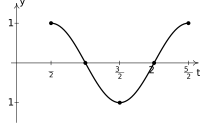
Figure 11.119
$g (t) = - \sin (t + \frac{π}{3})$ Period: $2 ⁢ π$ Amplitude: $1$ Phase Shift: $- \frac{π}{3}$ Vertical Shift: $0$
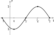
Figure 11.120
$h (t) = \sin (2 t - π)$ Period: $π$ Amplitude: $1$ Phase Shift: $\frac{π}{2}$ Vertical Shift: $0$
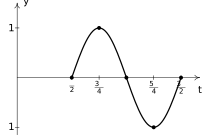
Figure 11.121
$f (t) = - \frac{1}{3} \cos (\frac{1}{2} t + \frac{π}{3})$ Period: $4 ⁢ π$ Amplitude: $\frac{1}{3}$ Phase Shift: $- \frac{2 π}{3}$ Vertical Shift: $0$
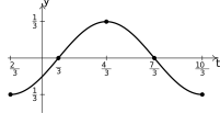
Figure 11.122
$g (t) = \cos (3 t - 2 π) + 4$ Period: $\frac{2 π}{3}$ Amplitude: $1$ Phase Shift: $\frac{2 π}{3}$ Vertical Shift: 4
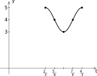
Figure 11.123
$h (t) = \sin (- t - \frac{π}{4}) - 2$ Period: $2 ⁢ π$ Amplitude: $1$ Phase Shift: $- \frac{π}{4}$ (You need to use $y = - \sin (t + \frac{π}{4}) - 2$ to find this.)²⁷ Vertical Shift: $minus 2$
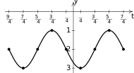
Figure 11.124
$f (t) = \frac{2}{3} \cos (\frac{π}{2} - 4 t) + 1$ Period: $\frac{π}{2}$ Amplitude: $\frac{2}{3}$ Phase Shift: $\frac{π}{8}$ (You need to use $y = \frac{2}{3} \cos (4 t - \frac{π}{2}) + 1$ to find this.)²⁸ Vertical Shift: $1$
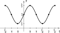
Figure 11.125
$g (t) = - \frac{3}{2} \cos (2 t + \frac{π}{3}) - \frac{1}{2}$ Period: $π$ Amplitude: $\frac{3}{2}$ Phase Shift: $- \frac{π}{6}$ Vertical Shift: $- \frac{1}{2}$
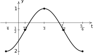
Figure 11.126
$h (t) = 4 \sin (- 2 π t + π)$ Period: $1$ Amplitude: $4$ Phase Shift: $\frac{1}{2}$ (You need to use $h (t) = - 4 \sin (2 π t - π)$ to find this.)²⁹ Vertical Shift: $0$
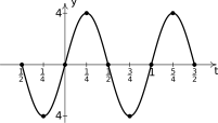
Figure 11.127
$S (t) = 4 \sin (t + \frac{π}{4})$ , $C (t) = 4 \cos (t - \frac{π}{4})$
$S (t) = - 3 \sin (t) + 3$ , $C (t) = - 3 \cos (t - \frac{π}{2}) + 3$
$S (t) = 3 \sin (2 t - \frac{π}{3})$ , $C (t) = 3 \cos (2 t - \frac{5 π}{6})$
$S (t) = \frac{7}{2} \sin (π t) + \frac{1}{2}$ , $C (t) = \frac{7}{2} \cos (π t \frac{π}{2}) + \frac{1}{2}$
1. $y equals vertical bar 4 ⁢ sin ⁡ open parenthesis t close parenthesis vertical bar$ . Period: $π$ .
  Two cycles are graphed below.
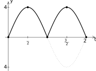
  Figure 11.128
2. $y = \sqrt{4 \sin (t)}$ . Period: $2 ⁢ π$ .
  One cycle is graphed below.
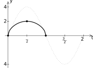
  Figure 11.129
$f (t) = \cos (3 t) + \sin (t)$ has period $2 ⁢ π$ .
The graph of $f (t) = t \sin (t)$ is bounded by the lines $y = \pm t$ ; $f$ has a variable amplitude of $t$ .
The graph of $f (t) = \frac{\sin (t)}{t}$ is bounded by the graphs of $y = \pm \frac{1}{t}$ ; $f$ has a variable amplitude of $\frac{1}{t}$ .
1. $lim t → ∞ f ⁢ open parenthesis t close parenthesis equals 0$ . We have a horizontal asymptote $y equals 0$ .
2. Since $- \frac{1}{t} \leq \frac{\sin (t)}{t} \leq \frac{1}{t}$ , $lim t → ∞$ $(- \frac{1}{t})$ $equals lim t → ∞$ $\frac{1}{t} = 0$ , $lim t → ∞$ $\frac{\sin (t)}{t} = 0$ by the Squeeze Theorem.
Graph $f (t) = \cos (\frac{1}{t})$ .
1. $lim t → 0 f ⁢ open parenthesis t close parenthesis$ does not exist. We have infinitely many oscillations as $t → 0$ .
2. $lim t → ∞ f ⁢ open parenthesis t close parenthesis equals 1$ since as $t → ∞$ , $\frac{1}{t} \to 0$ . Since cosine is continuous, $\cos (\frac{1}{t}) \to \cos (0) = 1$ .
  We have a horizontal asymptote $y equals 1$ .
The graph of $f (t) = e^{- 0.1 t} (\cos (2 t) + \sin (2 t))$ lies between³⁰ the graphs of $y = \pm 2 e^{- 0.1 t}$ .
1. $lim t → ∞ f ⁢ open parenthesis t close parenthesis equals 0$ . We have a horizontal asymptote $y equals 0$ .
2. Since $- 2 e^{- 0.1 t} \leq e^{- 0.1 t} (\cos (2 t) + \sin (2 t)) \leq 2 e^{- 0.1 t}$ , $lim t → ∞$ $(- 2 e^{- 0.1 t})$ $equals lim t → ∞$ $2 e^{- 0.1 t} = 0$ , the Squeeze Theorem gives $lim t → ∞$ $e^{- 0.1 t} (\cos (2 t) + \sin (2 t)) = 0$ .
$S ⁢ open parenthesis t close parenthesis equals sin ⁡ open parenthesis 880 ⁢ π ⁢ t close parenthesis$
$V (t) = 220 \sqrt{2} \sin (120 π t)$
$h (t) = 67.5 \sin (\frac{π}{15} t - \frac{π}{2}) + 67.5$
$x (t) = 67.5 \cos (\frac{π}{15} t - \frac{π}{2}) = 67.5 \sin (\frac{π}{15} t)$
$h (t) = 28 \sin (\frac{2 π}{3} t - \frac{π}{2}) + 30$
1. $θ (t) = θ_{0} \sin (\sqrt{\frac{g}{l}} t + \frac{π}{2})$
2. $θ (t) = \frac{π}{12} \sin (4 π t + \frac{π}{2})$
1. $T (t) = 20.5 \sin (\frac{π}{6} t - π) + 53.5$
2. The model and data are graphed below. The sinusoid is shifted to the right of our data.
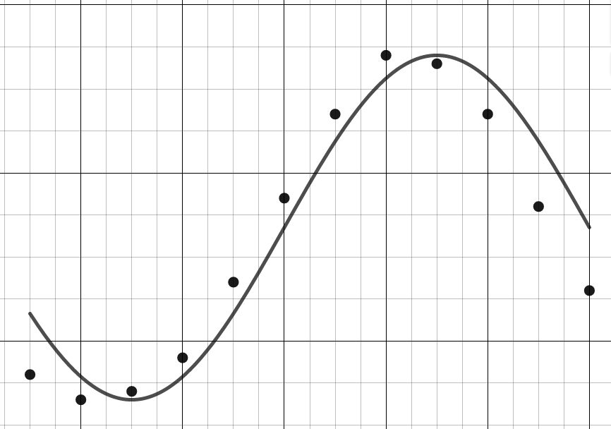
  Figure 11.130
3. The average temperature on April $15 to the power th$ is approximately $T ⁢ open parenthesis 4.5 close parenthesis approximately equals 39.00 degrees$ F and the average temperature on September $15 to the power th$ is approximately $T ⁢ open parenthesis 9.5 close parenthesis approximately equals 73.38 degrees$ F.
4. Desmos gives: $T (t) = 20.8374 \sin (- 0.5251 t - 0.2812) + 52.3659$ .
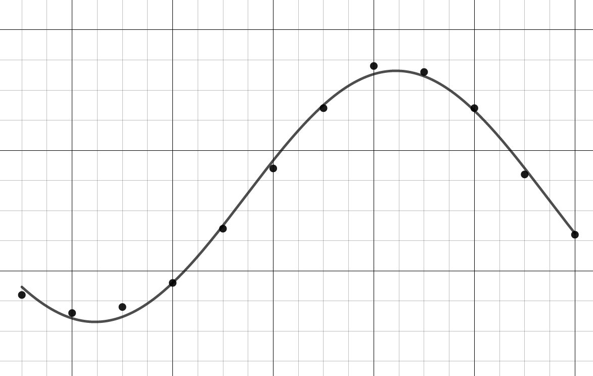
  Figure 11.131
  This model predicts the average temperature for April $15 to the power th$ to be approximately $42.42 degrees$ F and the average temperature on September $15 to the power th$ to be approximately $70.05 degrees$ F. This model appears to be more accurate.
1. Based on the shape of the data, we either choose $A less than 0$ or we find the second value of $t$ which closely approximates the `baseline' value, $F equals 0.505$ . We choose the latter to obtain $F (t) = 0.475 \sin (\frac{π}{15} t - 2 π) + 0.505 = 0.475 \sin (\frac{π}{15} t) + 0.505$
2. Our function and the data set are graphed below. It's a pretty good fit.
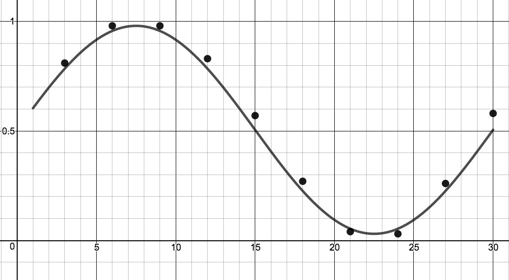
  Figure 11.132
3. The fraction of the moon illuminated on June 1st, 2009 is approximately $F ⁢ open parenthesis 1 close parenthesis approximately equals 0.60$
4. Using desmos,³¹ we get $F (t) = 0.49 \sin (\frac{π}{15} t - 6.29) + 0.535$ .
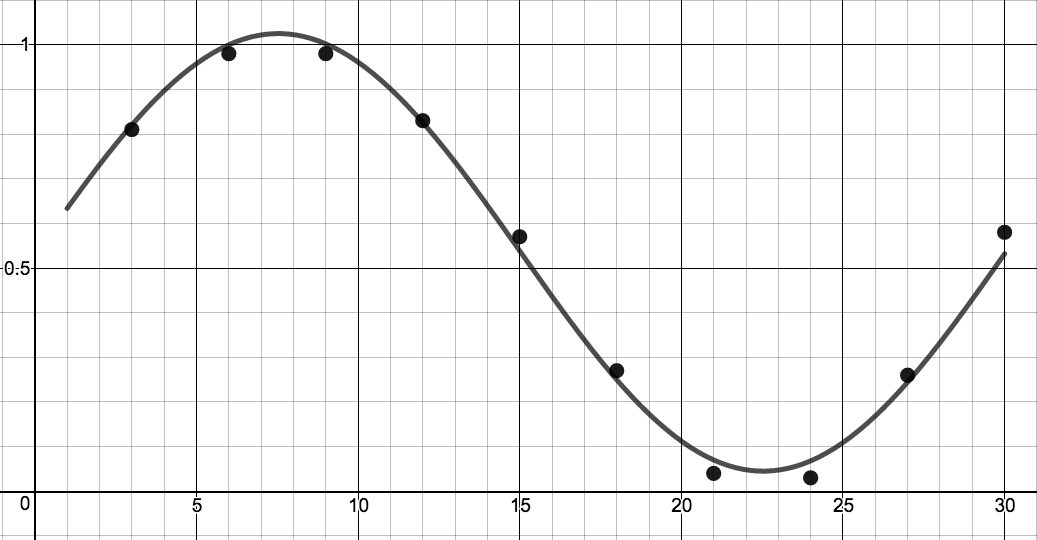
  Figure 11.133
  This model predicts that the fraction of the moon illuminated on June 1st, 2009 is approximately $0.63$ . This appears to be a better fit to the data than our first model.

which, you'll recall essentially `wraps the real number line around the Unit Circle ↩
in particular the interval $open bracket 0, 2 ⁢ π close parenthesis$ ↩
Keep in mind that we're using ` $y$ ' here to denote the output from the sine function. It is a coincidence that the $y$ -values on the graph of $y = \sin (t)$ correspond to the $y$ -values on the Unit Circle. ↩
Technically, we should study the interval $open bracket 0, 2 ⁢ π close parenthesis$ ,since whatever happens at $t equals 2 ⁢ π$ is the same as what happens at $t equals 0$ . As we will see shortly, $t equals 2 ⁢ π$ gives us an extra `check' when we go to graph these functions. ↩
Here note that the dependent variable ` $y$ ' represents the outputs from $g (t) = \cos (t)$ which are $x$ -coordinates on the Unit CIrcle. ↩
Hence, we can obtain the graph of $y = \sin (t)$ by shifting the graph of $y = \cos (t)$ to the right $\frac{π}{2}$ units: $\cos (t - \frac{π}{2}) = \sin (t)$ . ↩
this is the reason they are so useful in the Sciences and Engineering ↩
The reader may wish to review Definitions 2.2 and 2.3 as needed. ↩
See the remarks at the beginning of Section 5.4. ↩
If we use a linear function $f (t) = m t + b$ to transform the inputs, $t$ , then $Δ [f (t)] = m Δ t$ . That is, the change after the the transformation, $m Δ t$ , is just a multiple of the change before the transformation, $Δ t$ . ↩
If $t$ is time measured in seconds, then one cycle per second is 1 Hertz. ↩
Recall that velocity is speed with a direction. In 11.3, $ω greater than 0$ indicated counter-clockwise motion while $ω less than 0$ indicated clockwise motion. ↩
Note when we substitute the quarter marks into $f (t)$ , the argument of the cosine function simplifies to the quadrantal angles. That is, when we substitute $t equals 1$ , the argument of cosine simplifies to $0$ ; when we substitute $t equals 2$ , the argument simplifies $\frac{π}{2}$ and so on. This provides a quick check of our calculations. ↩
See Section 7.6. ↩
Otherwise, we could just observe the motion of the wheel from the other side. ↩
We are readjusting our `baseline' from $y equals 0$ to $y equals 72$ . ↩
Even though the data collected lies in the interval $open bracket 1, 12 close bracket$ , which has a length of $11$ , we need to think of the data point at $t equals 1$ as a representative sample of the amount of daylight for every day in January. That is, it represents $H (t)$ over the interval $open bracket 0, 1 close bracket$ . Similarly, $t equals 2$ is a sample of $H (t)$ over $open bracket 1, 2 close bracket$ , and so forth. ↩
See the figure on page Section 11.3. ↩
In Section 12.2, we can show how similar these two functions are analytically. See Exercise . ↩
See Exercises through in Section 11.4. ↩
Provided $θ$ is kept `small.' Carl remembers the `Rule of Thumb' as being $20 degrees$ or less. Check with your friendly neighborhood physicist to make sure. ↩
See this website: http://www.erh.noaa.gov/cle/climate/cle/normals/laketempcle.html. ↩
The computed average is $41 degrees$ F for April $15 to the power th$ and $71 degrees$ F for September $15 to the power th$ . ↩
See this website: http://www.usno.navy.mil/USNO/astronomical-applications/data-services/frac-moon-ill. ↩
You may want to plot the data before you find the phase shift. ↩
The listed fraction is $0.62$ . ↩
Two cycles of the graph are shown to illustrate the discrepancy discussed on page Section 11.3. ↩
Again, we graph two cycles to illustrate the discrepancy discussed on page Section 11.3. ↩
This will be the last time we graph two cycles to illustrate the discrepancy discussed on page Section 11.3. ↩
We'll be able to show in Section 12.2.1 that the graph of $f$ more perfectly lies between the graphs of $y = \pm \sqrt{2} e^{- 0.1 t}$ … ↩
…specifying $ω = \frac{π}{15}$ … ↩

Adapted from Precalculus, Preliminary 4th Edition (integrated calculus), by Carl Stitz and Jeff Zeager (stitz-zeager.com), licensed under CC BY-NC-SA 3.0. Changes were made: reformatted as an accessible XYZ web edition. License: CC-BY-NC-SA-3.0.