11.2 The Circular Functions: Sine and Cosine

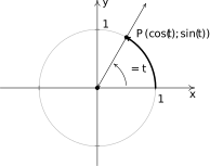
In Section 11.1.1, we introduced circular motion and derived a formula which describes the linear velocity of an object moving on a circular path at a constant angular velocity. One of the goals of this section is describe the position of such an object. To that end, consider an angle $θ$ in standard position and let $P$ denote the point where the terminal side of $θ$ intersects the Unit Circle, as diagrammed below.

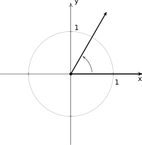
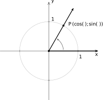
Coordinate-plane figure. — **Figure 11.39**

By associating the point $P$ with the angle $θ$ , we are assigning a position on the Unit Circle to the angle $θ$ . Since for each angle $θ$ , the terminal side of $θ$ , when graphed in standard position, intersects The Unit Circle only once, the mapping of $θ$ to $P$ is a function.¹ Since there is only one way to describe a point using rectangular coordinates,² the mappings of $θ$ to each of the $x$ and $y$ coordinates of $P$ are also functions. We give these functions names in the following definition.

Definition

Suppose an angle $θ$ is graphed in standard position. Let $P (x, y)$ be the point of intersection of the terminal side of $P$ and the Unit Circle.

The $x$ -coordinate of $P$ is called the cosine of $θ$ , written $\cos (θ)$ .
The $y$ -coordinate of $P$ is called the sine of $θ$ , written $\sin (θ)$ .³

You may have already seen definitions for the sine and cosine of an (acute) angle in terms of ratios of sides of a right triangle.⁴ While not incorrect, defining sine and cosine using right triangles limits the angles we can study to acute angles only. Definition 11.2, on the other hand, applies to all angles. Since these functions are defined in terms of points on the Unit Circle, they are called circular functions. Rest assured, Definition 11.2 specializes to Definition B.1 when $θ$ is an acute angle. We will see instances of this fact in the next example.

Example 1

Find the sine and cosine of the following angles.

$θ equals 270 degrees$
$θ = - π$
$θ equals 45 degrees$
$θ = \frac{π}{6}$
$θ = \frac{5 π}{6}$

To find $cos ⁡ open parenthesis 270 degrees close parenthesis$ and $sin ⁡ open parenthesis 270 degrees close parenthesis$ , we plot the angle $θ equals 270 degrees$ in standard position and find the point on the terminal side of $θ$ which lies on the Unit Circle. Since $270 degrees$ represents $\frac{3}{4}$ of a counter-clockwise revolution, the terminal side of $θ$ lies along the negative $y$ -axis. Hence, the point we seek is $open parenthesis 0, minus 1 close parenthesis$ so that $cos ⁡ open parenthesis 270 degrees close parenthesis equals 0$ and $\sin (270^{\circ}) = - 1$ .
The angle $θ = - π$ represents one half of a clockwise revolution so its terminal side lies on the negative $x$ -axis. The point on the Unit Circle that lies on the negative $x$ -axis is $open parenthesis minus 1, 0 close parenthesis$ which means $\cos (- π) = - 1$ and $\sin (- π) = 0$ .
Figure 11.41 Finding $cos ⁡ open parenthesis 270 degrees close parenthesis$ and $sin ⁡ open parenthesis 270 degrees close parenthesis$
Figure 11.42 Finding $\cos (- π)$ and $\sin (- π)$
In Section B.2, we derived values for $cos ⁡ open parenthesis 45 degrees close parenthesis$ and $sin ⁡ open parenthesis 45 degrees close parenthesis$ using Definition B.1. In order to connect what we know from Section B.2 with what we are asked to find per Definition 11.2, we sketch $θ equals 45 degrees$ in standard position and let $P (x, y)$ denote the point on the terminal side of $θ$ which lies on the Unit Circle. If we drop a perpendicular line segment from $P$ to the $x$ -axis as shown below on the left, we obtain a $45^{\circ} - 45^{\circ} - 90^{\circ}$ right triangle whose legs have lengths $x$ and $y$ units with hypotenuse $1$ . From our work in Section B.2, we obtain the (familiar) values $x = \cos (45^{\circ}) = \frac{\sqrt{2}}{2}$ and $y = \sin (45^{\circ}) = \frac{\sqrt{2}}{2}$ .
As before, the terminal side of $θ = \frac{π}{6}$ does not lie on any of the coordinate axes, so we proceed using a triangle approach. Letting $P (x, y)$ denote the point on the terminal side of $θ$ which lies on the Unit Circle, we drop a perpendicular line segment from $P$ to the $x$ -axis to form a $30^{\circ} - 60^{\circ} - 90^{\circ}$ right triangle. Re-using some of our work from Section B.2, we get $x = \cos (\frac{π}{6}) = \frac{\sqrt{3}}{2}$ and $y = \sin (\frac{π}{6}) = \frac{1}{2}$ .
Figure 11.43
Figure 11.44
We plot $θ = \frac{5 π}{6}$ in standard position below on the left and, as usual, let $P (x, y)$ denote the point on the terminal side of $θ$ which lies on the Unit Circle. In plotting $θ$ , we find it lies $\frac{π}{6}$ radians short of one half revolution. Since we've just determined that $\cos (\frac{π}{6}) = \frac{\sqrt{3}}{2}$ and $\sin (\frac{π}{6}) = \frac{1}{2}$ , we know the coordinates of the point $Q$ below on the right are $(\frac{\sqrt{3}}{2}, \frac{1}{2})$ . Using symmetry, the coordinates of $P$ are $(- \frac{\sqrt{3}}{2}, \frac{1}{2})$ , so $\cos (\frac{5 π}{6}) = - \frac{\sqrt{3}}{2}$ and $\sin (\frac{5 π}{6}) = \frac{1}{2}$ .
Figure 11.45
Figure 11.46

A few remarks are in order. First, after having re-used some of our work from Section B.2 in a few specific instances, we can reconcile Definition 11.2 with Definition B.1 in the case $θ$ is an acute angle. We situate $θ$ in a right triangle with hypotenuse length $1$ , adjacent side length ` $x$ ,' and the opposite side length ` $y$ ' as seen below on the left. Placing the vertex of $θ$ at the origin and the adjacent side of $θ$ along the $x$ -axis as seen below on the right effectively puts $θ$ in standard position with $θ$ 's adjacent side as the initial side of $θ$ and the hypotenuse as the terminal side of $θ$ . Since the hypotenuse of the triangle has length $1$ , we know the point $P (x, y)$ is on the Unit Circle.⁵

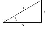
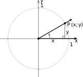
Definition B.1 gives $\cos (θ) = \frac{x}{1} = x$ and $\sin (θ) = \frac{y}{1} = y$ which exactly matches Definition 11.2. Hence, in the case of acute angles, the two definitions agree. In other words, the values of the trigonometric ratios of acute angles are the same as the corresponding circular function values.

A second important take-away from Example 11.2.1 is use of symmetry in number. Indeed, we found the sine and cosine of $\frac{5 π}{6}$ using the (acute) angle $\frac{π}{6}$ `for reference.' Since the Unit Circle is rife with symmetry, we would like to generalize this concept and exploit symmetry whenever possible. To that end, we introduce the notion of reference angle.

In general, for a non-quadrantal angle $θ$ , the reference angle for $θ$ (which we'll usually denote $α$ ) is the acute angle made between the terminal side of $θ$ and the $x$ -axis. If $θ$ is a Quadrant I or IV angle, $α$ is the angle between the terminal side of $θ$ and the positive $x$ -axis:

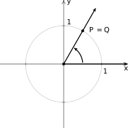
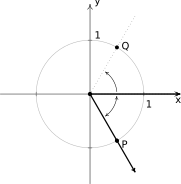
Reference angle $α$ for a Quadrant I angle

Reference angle $α$ for a Quadrant IV angle

If $θ$ is a Quadrant II or III angle, $α$ is the angle between the terminal side of $θ$ and the negative $x$ -axis:

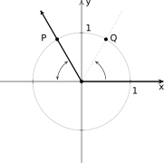
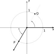
Reference angle $α$ for a Quadrant II angle

Reference angle $α$ for a Quadrant III angle

If we let $P$ denote the point $(\cos (θ), \sin (θ))$ , then $P$ lies on the Unit Circle. Since the Unit Circle possesses symmetry with respect to the $x$ -axis, $y$ -axis and origin, regardless of where the terminal side of $θ$ lies, there is a point $Q$ symmetric with $P$ which determines $θ$ 's reference angle, $α$ . The only difference between the points $P$ and $Q$ are the signs of their coordinates, $\pm$ . Hence, we have the following:

Theorem

Reference Angle Theorem. Suppose $α$ is the reference angle for $θ$ . Then:

$\cos (θ) = \pm \cos (α)$ and $\sin (θ) = \pm \sin (α)$ ,

where the choice of the ( $\pm$ ) depends on the quadrant in which the terminal side of $θ$ lies.

In light of Theorem 11.1, it pays to know the sine and cosine values for certain common Quadrant I angles as well as to keep in mind the signs of the coordinates of points in the given quadrants.

$\begin{matrix} θ (degrees) & θ (radians) & \cos (θ) & \sin (θ) \\ 0^{\circ} & 0 & 1 & 0 \\ 30^{\circ} & \frac{π}{6} & \frac{\sqrt{3}}{2} & \frac{1}{2} \\ 45^{\circ} & \frac{π}{4} & \frac{\sqrt{2}}{2} & \frac{\sqrt{2}}{2} \\ 60^{\circ} & \frac{π}{3} & \frac{1}{2} & \frac{\sqrt{3}}{2} \\ 90^{\circ} & \frac{π}{2} & 0 & 1 \end{matrix}$

Example 2

Find the sine and cosine of the following angles.

$θ equals 225 degrees$
$θ = \frac{11 π}{6}$
$θ = - \frac{5 π}{4}$
$θ = \frac{7 π}{3}$

We begin by plotting $θ equals 225 degrees$ in standard position and find its terminal side overshoots the negative $x$ -axis to land in Quadrant III. Hence, we obtain $θ$ 's reference angle $α$ by subtracting: $α = θ - 180^{\circ} = 225^{\circ} - 180^{\circ} = 45^{\circ}$ . Since $θ$ is a Quadrant III angle, both $cos ⁡ open parenthesis θ close parenthesis less than 0$ and $sin ⁡ open parenthesis θ close parenthesis less than 0$ . The Reference Angle Theorem yields: $\cos (225^{\circ}) = - \cos (45^{\circ}) = - \frac{\sqrt{2}}{2}$ and $\sin (225^{\circ}) = - \sin (45^{\circ}) = - \frac{\sqrt{2}}{2}$ .
The terminal side of $θ = \frac{11 π}{6}$ , when plotted in standard position, lies in Quadrant IV, just shy of the positive $x$ -axis. To find $θ$ 's reference angle $α$ , we subtract: $α = 2 π - θ = 2 π - \frac{11 π}{6} = \frac{π}{6}$ . Since $θ$ is a Quadrant IV angle, $cos ⁡ open parenthesis θ close parenthesis greater than 0$ and $sin ⁡ open parenthesis θ close parenthesis less than 0$ , so the Reference Angle Theorem gives: $\cos (\frac{11 π}{6}) = \cos (\frac{π}{6}) = \frac{\sqrt{3}}{2}$ and $\sin (\frac{11 π}{6}) = - \sin (\frac{π}{6}) = - \frac{1}{2}$ .
Figure 11.54 Finding $cos ⁡ open parenthesis 225 degrees close parenthesis$ and $sin ⁡ open parenthesis 225 degrees close parenthesis$
Figure 11.55 Finding $\cos (\frac{11 π}{6})$ and $\sin (\frac{11 π}{6})$
To plot $θ = - \frac{5 π}{4}$ , we rotate clockwise an angle of $\frac{5 π}{4}$ from the positive $x$ -axis. The terminal side of $θ$ , therefore, lies in Quadrant II making an angle of $α = \frac{5 π}{4} - π = \frac{π}{4}$ radians with respect to the negative $x$ -axis. Since $θ$ is a Quadrant II angle, $cos ⁡ open parenthesis θ close parenthesis less than 0$ and $sin ⁡ open parenthesis θ close parenthesis greater than 0$ so the Reference Angle Theorem gives: $\cos (- \frac{5 π}{4}) = - \cos (\frac{π}{4}) = - \frac{\sqrt{2}}{2}$ and $\sin (- \frac{5 π}{4}) = \sin (\frac{π}{4}) = \frac{\sqrt{2}}{2}$ .
Since the angle $θ = \frac{7 π}{3}$ measures more than $2 π = \frac{6 π}{3}$ , we find the terminal side of $θ$ by rotating one full revolution followed by an additional $α = \frac{7 π}{3} - 2 π = \frac{π}{3}$ radians. Hence, $θ$ and $α$ have the same terminal side,⁶ and so $\cos (\frac{7 π}{3}) = \cos (\frac{π}{3}) = \frac{1}{2}$ and $\sin (\frac{7 π}{3}) = \sin (\frac{π}{3}) = \frac{\sqrt{3}}{2}$ .
Figure 11.56 Finding $\cos (- \frac{5 π}{4})$ and $\sin (- \frac{5 π}{4})$
Figure 11.57 Finding $\cos (\frac{7 π}{3})$ and $\sin (\frac{7 π}{3})$

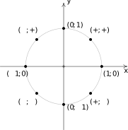
A couple of remarks are in order. First off, the reader may have noticed that when expressed in radian measure, the reference angle for a non-quadrantal angle is easy to spot. Reduced fraction multiples of $π$ with a denominator of $6$ have $\frac{π}{6}$ as a reference angle, those with a denominator of $4$ have $\frac{π}{4}$ as their reference angle, and those with a denominator of $3$ have $\frac{π}{3}$ as their reference angle.⁷

Also note in number above, the angles $\frac{π}{3}$ and $\frac{7 π}{3}$ are coterminal. As a result, have the same values for sine and cosine. It turns out that we can characterize coterminal angles in this manner, as stated below.

Theorem

Two angles $α$ and $β$ are coterminal if and only if:

$\cos (α) = \cos (β)$ and $\sin (α) = \sin (β)$ .

Recall the phraseology `if and only if' means there are two things to argue in Theorem 11.2: first, if $α$ and $β$ are co-terminal, then $\cos (α) = \cos (β)$ and $\sin (α) = \sin (β)$ . This is immediate since coterminal share terminal sides, and, in particular, the (unique) point on the Unit Circle shared by said terminal side. Second, we need to argue that if $\cos (α) = \cos (β)$ and $\sin (α) = \sin (β)$ , then $α$ and $β$ are coterminal.

To prove this second claim, note that when an angle is drawn in standard position, the terminal side of the angle is the ray that starts at the origin and is completely determined by any other point on the terminal side. If $\cos (α) = \cos (β)$ and $\sin (α) = \sin (β)$ , then their terminal sides share a point on the Unit Circle, namely $(\cos (α), \sin (α)) = (\cos (β), \sin (β))$ . Hence, $α$ and $β$ are coterminal.

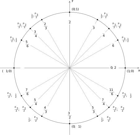
The Reference Angle Theorem in conjunction with the table of sine and cosine values on Page Section 11.2 can be used to generate the figure on the next page. We recommend committing it to memory.

Figure: Important Points on the Unit Circle — **Figure 11.58** Important Points on the Unit Circle

Our next example uses The Reference Angle Theorem in a slightly more sophisticated context.

Example 3

Suppose $α$ is an acute angle with $\cos (α) = \frac{5}{13}$ .

Find $\sin (α)$ and use this to plot $α$ in standard position.
Find the sine and cosine of the following angles:
1. $θ = π + α$
2. $θ = 2 π - α$
3. $θ = 3 π - α$
4. $θ = \frac{π}{2} + α$

Since $α$ is an acute angle, we know $0 < α < \frac{π}{2}$ so the terminal side of $α$ lies in Quadrant I. Moreover, since $\cos (α) = \frac{5}{13}$ , we know the $x$ -coordinate of the intersection point of the terminal side of $α$ and the Unit Circle is $\frac{5}{13}$ . To find $\sin (α)$ , we need the $y$ -coordinate. Taking a cue from Example 11.2.1, we drop a perpendicular from the terminal side of $α$ to the $x$ -axis as seen below on the right to form a right triangle with one leg measuring $\frac{5}{13}$ units and hypotenuse with a length of $1$ unit.
Figure 11.59
Figure 11.60
The Pythagorean Theorem gives ${(\frac{5}{13})}^{2} + y^{2} = 1^{2}$ or $y = \frac{12}{13}$ . Hence, $\sin (α) = \frac{12}{13}$ .
1. To find the cosine and sine of $θ = π + α$ , we first plot $θ$ in standard position. We can imagine the sum of the angles $π + α$ as a sequence of two rotations: a rotation of $π$ radians followed by a rotation of $α$ radians.⁸ We see that $α$ is the reference angle for $θ$ . By The Reference Angle Theorem, $\cos (θ) = \pm \cos (α) = \pm \frac{5}{13}$ and $\sin (θ) = \pm \sin (α) = \pm \frac{12}{13}$ . Since the terminal side of $θ$ falls in Quadrant III, both $\cos (θ)$ and $\sin (θ)$ are negative, so $\cos (θ) = - \frac{5}{13}$ and $\sin (θ) = - \frac{12}{13}$ .
  Figure 11.61 Visualizing $θ = π + α$
  Figure 11.62 $θ$ has reference angle $α$
2. Rewriting $θ = 2 π - α$ as $θ = 2 π + (- α)$ , we can plot $θ$ by visualizing one complete revolution counter-clockwise followed by a clockwise revolution, or `backing up,' of $α$ radians. Once again, we see that $α$ is $θ$ 's reference angle. Since $θ$ is a Quadrant IV angle, we choose the appropriate signs and get: $\cos (θ) = \frac{5}{13}$ and $\sin (θ) = - \frac{12}{13}$ .
  Figure 11.63 Visualizing $θ = 2 π - α$
  Figure 11.64 $θ$ has reference angle $α$
3. Taking a cue from the previous problem, we rewrite $θ = 3 π - α$ as $θ = 3 π + (- α)$ . The angle $3 ⁢ π$ represents one and a half revolutions counter-clockwise, so that when we `back up' $α$ radians, we end up in Quadrant II. Since $α$ is the reference angle for $θ$ , The Reference Angle Theorem gives $\cos (θ) = - \frac{5}{13}$ and $\sin (θ) = \frac{12}{13}$ .
  Figure 11.65 Visualizing $3 ⁢ π minus α$
  Figure 11.66 $θ$ has reference angle $α$
4. To plot $θ = \frac{π}{2} + α$ , we first rotate $\frac{π}{2}$ radians and follow up with $α$ radians. The reference angle here is not $α$ , so The Reference Angle Theorem is not immediately applicable. (It's important that you see why this is the case. Take a moment to think about this before reading on.) Let $Q (x, y)$ be the point on the terminal side of $θ$ which lies on the Unit Circle so that $x = \cos (θ)$ and $y = \sin (θ)$ . Once we graph $α$ in standard position, we use the fact from Geometry that equal angles subtend equal chords to show that the dotted lines in the figure below are equal. Hence, $x = \cos (θ) = - \frac{12}{13}$ . Similarly, we find $y = \sin (θ) = \frac{5}{13}$ .
  Figure 11.67 Visualizing $θ = \frac{π}{2} + α$
  Figure 11.68

A couple of remarks about Example 11.2.3 are in order. First, we note the right triangle we used to find $\sin (α)$ is a scaled 5-12-13 triangle. Recognizing this Pythagorean Triple⁹ may have simplified our workflow. Along the same lines, since, the Unit Circle, by definition, is described by the equation $x^{2} + y^{2} = 1$ , we could substitute $x = \frac{5}{13}$ in order to find $y$ . We leave it to the reader to show we get the exact same answer regardless of the approach used.

Our next example turns the tables and makes good use of the Unit Circle values given on Section 11.2 as well as Theorem 11.2 in a different way: instead of giving information about the angle and asking for sine or cosine values, we are given sine or cosine values and asked to produce the corresponding angles. In other words, we solve some rudimentary equations involving sine and cosine.¹⁰

Example 4

Find all angles that satisfy the following equations. Express your answers in radians.¹¹

$\cos (θ) = \frac{1}{2}$
$\sin (α) = - \frac{1}{2}$
$cos ⁡ open parenthesis β close parenthesis equals 0$ .
$\sin (γ) = \frac{3}{2}$

If $\cos (θ) = \frac{1}{2}$ , then we know the terminal side of $θ$ , when plotted in standard position, intersects the Unit Circle at $x = \frac{1}{2}$ . This means $θ$ is a Quadrant I or IV angle. Since $\cos (θ) = \frac{1}{2}$ , we know from the values on page Section 11.2 that the reference angle is $\frac{π}{3}$ .
Figure 11.69
Figure 11.70
One solution in Quadrant I is $θ = \frac{π}{3}$ . Per Theorem 11.2, all other Quadrant I solutions must be coterminal with $\frac{π}{3}$ . Recall from Section 11.1, two angles in radian measure are coterminal if and only if they differ by an integer multiple of $2 ⁢ π$ . Hence to describe all angles coterminal with a given angle, we add $2 ⁢ π ⁢ k$ for integers $k equals 0$ , $\pm 1$ , $\pm 2$ , …. Hence, we record our final answer as $θ = \frac{π}{3} + 2 π k$ for integers $k$ . Proceeding similarly for the Quadrant IV case, we find the solution to $\cos (θ) = \frac{1}{2}$ here is $\frac{5 π}{3}$ , so our answer in this Quadrant is $θ = \frac{5 π}{3} + 2 π k$ for integers $k$ .
If $\sin (α) = - \frac{1}{2}$ , then when $α$ is plotted in standard position, its terminal side intersects the Unit Circle at $y = - \frac{1}{2}$ . From this, we determine $α$ is a Quadrant III or Quadrant IV angle with reference angle $\frac{π}{6}$ . In Quadrant III, one solution is $\frac{7 π}{6}$ , so we capture all Quadrant III solutions by adding integer multiples of $2 ⁢ π$ : $α = \frac{7 π}{6} + 2 π k$ . In Quadrant IV, one solution is $\frac{11 π}{6}$ so all the solutions here are of the form $α = \frac{11 π}{6} + 2 π k$ for integers $k$ .
Figure 11.71
Figure 11.72
If $cos ⁡ open parenthesis β close parenthesis equals 0$ , then the terminal side of $β$ must lie on the line $x equals 0$ , also known as the $y$ -axis.
Figure 11.73
Figure 11.74
While, technically speaking, $\frac{π}{2}$ isn't a reference angle (it's not acute), we can nonetheless use it to find our answers. If we follow the procedure set forth in the previous examples, we find $β = \frac{π}{2} + 2 π k$ and $β = \frac{3 π}{2} + 2 π k$ for integers, $k$ . While this solution is correct, it can be shortened to $β = \frac{π}{2} + π k$ for integers $k$ . The reader is encouraged to see the geometry using the diagram above on the left.
We are asked to solve $\sin (γ) = \frac{3}{2}$ . Since sine values are $y$ -coordinates on the Unit Circle, $\sin (γ)$ can't be any larger than $1$ . Hence, $\sin (t) = \frac{3}{2}$ has no solutions.

One of the key items to take from Example 11.2.4 is that, in general, solutions to trigonometric equations consist of infinitely many answers. To get a feel for these answers, the reader is encouraged to follow our mantra from Chapter 10 - that is, `When in doubt, write it out!' This is especially important when checking answers to the exercises.

For example, another Quadrant IV solution to $\sin (θ) = - \frac{1}{2}$ is $θ = - \frac{π}{6}$ . Hence, the family of Quadrant IV answers to number above could just have easily been written $θ = - \frac{π}{6} + 2 π k$ for integers $k$ . While on the surface, this family may look different than the stated solution of $θ = \frac{11 π}{6} + 2 π k$ for integers $k$ , we leave it to the reader to show they represent the same list of angles.

It is also worth noting that when asked to solve equations in algebra, we are usually looking for real number solutions. Thanks to the identifications made on page Section 11.1, we are able to regard the inputs to the sine and cosine functions as real numbers by identifying any real number $t$ with an oriented angle $θ$ measuring $θ = t$ radians. That is, for each real number $t$ , we associate an oriented arc $t$ units in length with initial point $open parenthesis 1, 0 close parenthesis$ and endpoint $P (\cos (t), \sin (t))$ .

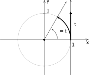
In practice this means in expressions like ` $\cos (π)$ ' and ` $sin ⁡ open parenthesis 2 close parenthesis$ ,' the inputs can be thought of as either angles in radian measure or real numbers, whichever is more convenient.

Suppose, as in the Exercises, we are asked to find all real number solutions to the equation such as $\sin (t) = - \frac{1}{2}$ . The discussion above allows us to find the real number solutions to this equation by thinking in angles. Indeed, we would solve this equation in the exact way we solved $\sin (θ) = - \frac{1}{2}$ in Example 11.2.4 number. Our solution is only cosmetically different in that the variable used is $t$ rather than $θ$ : $t = \frac{7 π}{6} + 2 π k$ or $t = \frac{11 π}{6} + 2 π k$ for integers, $k$ .

We will study the sine and cosine functions in greater detail in Section 11.3. Until then, keep in mind that any properties of the sine and cosine functions developed in the following sections which regard them as functions of angles in radian measure apply equally well if the inputs are regarded as real numbers.

Beyond the Unit Circle

In Definition 11.2, we define the sine and cosine functions using the Unit Circle, $x^{2} + y^{2} = 1$ . It turns out that we can use any circle centered at the origin to determine the sine and cosine values of angles. To show this, we essentially recycle the same similarity arguments used in Section B.2 to show the trigonometric ratios described in Definition B.1 are independent of the choice of right triangle used.¹²

Consider for the moment the acute angle $θ$ drawn below in standard position. Let $Q (x, y)$ be the point on the terminal side of $θ$ which lies on the circle $x^{2} + y^{2} = r^{2}$ , and let $P (x^{'}, y^{'})$ be the point on the terminal side of $θ$ which lies on the Unit Circle. Now consider dropping perpendiculars from $P$ and $Q$ to create two right triangles, $Δ O P A$ and $Δ O Q B$ . These triangles are similar,¹³ thus it follows that $\frac{x}{x^{'}} = \frac{r}{1} = r$ , so $x = r x^{'}$ and, similarly, we find $y = r y^{'}$ . Since, by definition, $x^{'} = \cos (θ)$ and $y^{'} = \sin (θ)$ , we get the coordinates of $Q$ to be $x = r \cos (θ)$ and $y = r \sin (θ)$ . By reflecting these points through the $x$ -axis, $y$ -axis and origin, we obtain the result for all non-quadrantal angles $θ$ , and we leave it to the reader to verify these formulas hold for the quadrantal angles as well.

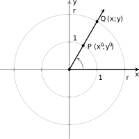
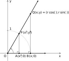
Not only can we describe the coordinates of $Q$ in terms of $\cos (θ)$ and $\sin (θ)$ but since the radius of the circle is $r = \sqrt{x^{2} + y^{2}}$ , we can also express $\cos (θ)$ and $\sin (θ)$ in terms of the coordinates of $Q$ . These results are summarized in the following theorem.

Theorem

If $Q (x, y)$ is the point on the terminal side of an angle $θ$ , plotted in standard position, which lies on the circle $x^{2} + y^{2} = r^{2}$ then $x = r \cos (θ)$ and $y = r \sin (θ)$ . Moreover,

$\begin{matrix} \cos (θ) = \frac{x}{r} = \frac{x}{\sqrt{x^{2} + y^{2}}} & and & \sin (θ) = \frac{y}{r} = \frac{y}{\sqrt{x^{2} + y^{2}}} \end{matrix}$

Note that in the case of the Unit Circle we have $r = \sqrt{x^{2} + y^{2}} = 1$ , so Theorem 11.3 reduces to our definitions of $\cos (θ)$ and $\sin (θ)$ in Definition 11.2. Our next example makes good use of Theorem 11.3.

Example 5

Suppose that the terminal side of an angle $θ$ , when plotted in standard position, contains the point $Q ⁢ open parenthesis 4, minus 2 close parenthesis$ . Find $\sin (θ)$ and $\cos (θ)$ .
Suppose $\frac{π}{2} < θ < π$ with $\sin (θ) = \frac{8}{17}$ . Find $\cos (θ)$ .
In Example 11.1.3 in Section 11.1, we approximated the radius of the earth at $41.628 degrees$ north latitude to be $2960$ miles. Justify this approximation if the spherical radius of the Earth is $3960$ miles.

Since we are given both the $x$ and $y$ coordinates of a point on the terminal side of this angle, we can use Theorem 11.3 directly. First, we find $r = \sqrt{x^{2} + y^{2}} = \sqrt{{(- 2)}^{2} + 4^{2}} = \sqrt{20} = 2 \sqrt{5}$ . This means the point $Q$ lies on a circle of radius $2 ⁢ the square root of 5$ units as seen below on the left. Hence, $\cos (θ) = \frac{x}{r} = \frac{4}{2 \sqrt{5}} = \frac{2 \sqrt{5}}{5}$ and $\sin (θ) = \frac{y}{r} = \frac{- 2}{2 \sqrt{5}} = - \frac{\sqrt{5}}{5}$ .
We are told $\frac{π}{2} < θ < π$ , so, in particular, $θ$ is a Quadrant II angle. Per Theorem 11.3, $\sin (θ) = \frac{8}{17} = \frac{y}{r}$ where $y$ is the $y$ -coordinate of the intersection point of the circle $x^{2} + y^{2} = r^{2}$ and the terminal side of $θ$ (when plotted in standard position, of course!) For convenience, we choose $r equals 17$ so that $y equals 8$ , and we get the diagram below on the right. Since $x^{2} + y^{2} = r^{2}$ , we get $x^{2} + 8^{2} = 17^{2}$ . We find $x = \pm 15$ , and since $θ$ is a Quadrant II angle, we get $x = - 15$ . Hence, $\cos (θ) = - \frac{15}{17}$ .
Figure 11.79 $Q ⁢ open parenthesis 4, minus 2 close parenthesis$ lies on a circle of radius $2 ⁢ the square root of 5$ units
Figure 11.80 $0 < θ < \frac{π}{2}$ with $\sin (θ) = \frac{8}{17}$
Recall the diagram below on the left indicating the circles which are the parallels of latitude.¹⁴
Figure 11.81
Figure 11.82

Assuming the Earth is a sphere of radius $3960$ miles, a cross-section through the poles produces a circle of radius $3960$ miles. Viewing the Equator as the $x$ -axis, the value we seek is the $x$ -coordinate of the point $Q (x, y)$ indicated in the figure above on the right. Using Theorem 11.3, we get $x = 3960 \cos ({41.628}^{\circ}) \approx 2960$ . Hence, the radius of the Earth at North Latitude $41.628 degrees$ is approximately $2960$ miles.

Theorem 11.3 gives us what we need to `circle back' to the question posed at the the beginning of the section: how to describe the position of an object traveling in a circular path of radius $r$ with constant angular velocity $ω$ . Suppose that at time $t$ , the object has swept out an angle measuring $θ$ radians. If we assume that the object is at the point $open parenthesis r, 0 close parenthesis$ when $t equals 0$ , the angle $θ$ is in standard position. By definition, $ω = \frac{θ}{t}$ which we rewrite as $θ = ω t$ . According to Theorem 11.3, the location of the object $Q (x, y)$ on the circle is found using the equations $x = r \cos (θ) = r \cos (ω t)$ and $y = r \sin (θ) = r \sin (ω t)$ . Hence, at time $t$ , the object is at the point $(r \cos (ω t), r \sin (ω t))$ , as seen in the diagram below.

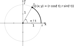
Equations for Circular Motion

We have just argued the following.

Equation

Suppose an object is traveling in a circular path of radius $r$ centered at the origin with constant angular velocity $ω$ . If $t equals 0$ corresponds to the point $open parenthesis r, 0 close parenthesis$ , then the $x$ and $y$ coordinates of the object are functions of $t$ and are given by $x = r \cos (ω t)$ and $y = r \sin (ω t)$ . Here, $ω greater than 0$ indicates a counter-clockwise direction and $ω less than 0$ indicates a clockwise direction.

Example 6

Suppose we are in the situation of Example 11.1.3. Find the equations of motion of Lakeland Community College as the earth rotates.

From Example 11.1.3, we take $r equals 2960$ miles and and $ω = \frac{π}{12 hours}$ . Hence, the equations of motion are $x = r \cos (ω t) = 2960 \cos (\frac{π}{12} t)$ and $y = r \sin (ω t) = 2960 \sin (\frac{π}{12} t)$ , where $x$ and $y$ are measured in miles and $t$ is measured in hours.¹⁵

Exercises

In Exercises -, find the exact value of the cosine and sine of the given angle.

$θ equals 0$
$θ = \frac{π}{4}$
$θ = \frac{π}{3}$
$θ = \frac{π}{2}$
$θ = \frac{2 π}{3}$
$θ = \frac{3 π}{4}$
$θ = π$
$θ = \frac{7 π}{6}$
$θ = \frac{5 π}{4}$
$θ = \frac{4 π}{3}$
$θ = \frac{3 π}{2}$
$θ = \frac{5 π}{3}$
$θ = \frac{7 π}{4}$
$θ = \frac{23 π}{6}$
$θ = - \frac{13 π}{2}$
$θ = - \frac{43 π}{6}$
$θ = - \frac{3 π}{4}$
$θ = - \frac{π}{6}$
$θ = \frac{10 π}{3}$
$θ equals 117 ⁢ π$

In Exercises -, find all of the angles which satisfy the given equation.

$\sin (θ) = \frac{1}{2}$
$\cos (θ) = - \frac{\sqrt{3}}{2}$
$sin ⁡ open parenthesis θ close parenthesis equals 0$
$\cos (θ) = \frac{\sqrt{2}}{2}$
$\sin (θ) = \frac{\sqrt{3}}{2}$
$\cos (θ) = - 1$
$\sin (θ) = - 1$
$\cos (θ) = \frac{\sqrt{3}}{2}$
$\cos (θ) = - 1.001$

In Exercises -, solve the equation for $t$ . (See the remarks on page Section 11.2.)

$cos ⁡ open parenthesis t close parenthesis equals 0$
$\sin (t) = - \frac{\sqrt{2}}{2}$
$cos ⁡ open parenthesis t close parenthesis equals 3$
$\sin (t) = - \frac{1}{2}$
$\cos (t) = \frac{1}{2}$
$\sin (t) = - 2$
$cos ⁡ open parenthesis t close parenthesis equals 1$
$sin ⁡ open parenthesis t close parenthesis equals 1$
$\cos (t) = - \frac{\sqrt{2}}{2}$

In Exercises -, let $θ$ be the angle in standard position whose terminal side contains the given point then compute $\cos (θ)$ and $\sin (θ)$ .

$P ⁢ open parenthesis minus 7, 24 close parenthesis$
$Q ⁢ open parenthesis 3, 4 close parenthesis$
$R ⁢ open parenthesis 5, minus 9 close parenthesis$
$T (- 2, - 11)$

In Exercises -, use the results developed throughout the section to find the requested value.

If $\sin (θ) = - \frac{7}{25}$ with $θ$ in Quadrant IV, what is $\cos (θ)$ ?
If $\cos (θ) = \frac{4}{9}$ with $θ$ in Quadrant I, what is $\sin (θ)$ ?
If $\sin (θ) = \frac{5}{13}$ with $θ$ in Quadrant II, what is $\cos (θ)$ ?
If $\cos (θ) = - \frac{2}{11}$ with $θ$ in Quadrant III, what is $\sin (θ)$ ?
If $\sin (θ) = - \frac{2}{3}$ with $θ$ in Quadrant III, what is $\cos (θ)$ ?
If $\cos (θ) = \frac{28}{53}$ with $θ$ in Quadrant IV, what is $\sin (θ)$ ?
If $\sin (θ) = \frac{2 \sqrt{5}}{5}$ and $\frac{π}{2} < θ < π$ , what is $\cos (θ)$ ?
If $\cos (θ) = \frac{\sqrt{10}}{10}$ and $2 π < θ < \frac{5 π}{2}$ , what is $\sin (θ)$ ?
If $\sin (θ) = - 0.42$ and $π < θ < \frac{3 π}{2}$ , what is $\cos (θ)$ ?
If $\cos (θ) = - 0.98$ and $\frac{π}{2} < θ < π$ , what is $\sin (θ)$ ?

In Exercises -, use your calculator to approximate the given value to three decimal places. Make sure your calculator is in the proper angle measurement mode!

$sin ⁡ open parenthesis 78.95 degrees close parenthesis$
$cos ⁡ open parenthesis minus 2.01 close parenthesis$
$sin ⁡ open parenthesis 392.994 close parenthesis$
$cos ⁡ open parenthesis 207 degrees close parenthesis$
$\sin (π^{\circ})$
$\cos (e)$

In Exercises -, write the given function as a nontrivial decomposition of functions as directed.

For $f (t) = 3 t + \sin (2 t)$ , find functions $g$ and $h$ so that $f = g + h$ .
For $f (θ) = 3 \cos (θ) - \sin (4 θ)$ , find functions $g$ and $h$ so that $f = g - h$ .
For $f (t) = e^{- 0.1 t} \sin (3 t)$ , find functions $g$ and $h$ so that $f = g h$ .
For $r (t) = \frac{\sin (t)}{t}$ , find functions $f$ and $g$ so $r = \frac{f}{g}$ .
For $r (θ) = \sqrt{3 \cos (θ)}$ , find functions $f$ and $g$ so $r equals g ∘ f$ .
For each function $S (t)$ listed below, compute the average rate of change over the indicated interval.¹⁶ What trends do you notice? Be sure your calculator is in radian mode!
$\begin{matrix} S (t) & [- 0.1, 0.1] & [- 0.01, 0.01] & [- 0.001, 0.001] \\ \sin (t) \\ \sin (2 t) \\ \sin (3 t) \\ \sin (4 t) \end{matrix}$

In Exercises -, find the equations of motion for the given scenario. Assume that the center of the motion is the origin, the motion is counter-clockwise and that $t equals 0$ corresponds to a position along the positive $x$ -axis. (See Equation 11.3 and Example 11.1.3.)

A point on the edge of the spinning yo-yo in Exercise from Section 11.1.
Recall: The diameter of the yo-yo is 2.25 inches and it spins at 4500 revolutions per minute.
The yo-yo in exercise from Section 11.1.
Recall: The radius of the circle is 28 inches and it completes one revolution in 3 seconds.
A point on the edge of the hard drive in Exercise from Section 11.1.
Recall: The diameter of the hard disk is 2.5 inches and it spins at 7200 revolutions per minute.
A passenger on the Big Wheel in Exercise from Section 11.1.
Recall: The diameter is 128 feet and completes 2 revolutions in 2 minutes, 7 seconds.
Consider the numbers: $0$ , $1$ , $2$ , $3$ , $4$ . Take the square root of each of these numbers, then divide each by $2$ . The resulting numbers should look hauntingly familiar. (See the values in the table on Section 11.2.)
On page Section 11.2, we see that the sine and cosine functions of angles can be considered functions of real numbers. With help from your classmates, discuss the domains and ranges of $f (t) = \sin (t)$ and $g (t) = \cos (t)$ . Write your answers using interval notation.
Another way to establish Theorem 11.3 is to use transformations. Re-read the discussion following Theorem 8.4 in Chapter 8 and transform the Unit Circle, $x^{2} + y^{2} = 1$ , to $x^{2} + y^{2} = r^{2}$ using horizontal and vertical stretches. Show if the coordinates on the Unit Circle are $(\cos (θ), \sin (θ))$ , then the corresponding coordinates on $x^{2} + y^{2} = r^{2}$ are $(r \cos (θ), r \sin (θ))$ .
In the scenario of Equation 11.3, we assumed that at $t equals 0$ , the object was at the point $open parenthesis r, 0 close parenthesis$ . If this is not the case, we can adjust the equations of motion by introducing a `time delay.' If $t sub 0 greater than 0$ is the first time the object passes through the point $open parenthesis r, 0 close parenthesis$ , show, with the help of your classmates, the equations of motion are $x = r \cos (ω (t - t_{0}))$ and $y = r \sin (ω (t - t_{0}))$ .

Answers

$cos ⁡ open parenthesis 0 close parenthesis equals 1$ , $sin ⁡ open parenthesis 0 close parenthesis equals 0$
$\cos (\frac{π}{4}) = \frac{\sqrt{2}}{2}$ , $\sin (\frac{π}{4}) = \frac{\sqrt{2}}{2}$
$\cos (\frac{π}{3}) = \frac{1}{2}$ , $\sin (\frac{π}{3}) = \frac{\sqrt{3}}{2}$
$\cos (\frac{π}{2}) = 0$ , $\sin (\frac{π}{2}) = 1$
$\cos (\frac{2 π}{3}) = - \frac{1}{2}$ , $\sin (\frac{2 π}{3}) = \frac{\sqrt{3}}{2}$
$\cos (\frac{3 π}{4}) = - \frac{\sqrt{2}}{2}$ , $\sin (\frac{3 π}{4}) = \frac{\sqrt{2}}{2}$
$\cos (π) = - 1$ , $sin ⁡ open parenthesis π close parenthesis equals 0$
$\cos (\frac{7 π}{6}) = - \frac{\sqrt{3}}{2}$ , $\sin (\frac{7 π}{6}) = - \frac{1}{2}$
$\cos (\frac{5 π}{4}) = - \frac{\sqrt{2}}{2}$ , $\sin (\frac{5 π}{4}) = - \frac{\sqrt{2}}{2}$
$\cos (\frac{4 π}{3}) = - \frac{1}{2}$ , $\sin (\frac{4 π}{3}) = - \frac{\sqrt{3}}{2}$
$\cos (\frac{3 π}{2}) = 0$ , $\sin (\frac{3 π}{2}) = - 1$
$\cos (\frac{5 π}{3}) = \frac{1}{2}$ , $\sin (\frac{5 π}{3}) = - \frac{\sqrt{3}}{2}$
$\cos (\frac{7 π}{4}) = \frac{\sqrt{2}}{2}$ , $\sin (\frac{7 π}{4}) = - \frac{\sqrt{2}}{2}$
$\cos (\frac{23 π}{6}) = \frac{\sqrt{3}}{2}$ , $\sin (\frac{23 π}{6}) = - \frac{1}{2}$
$\cos (- \frac{13 π}{2}) = 0$ , $\sin (- \frac{13 π}{2}) = - 1$
$\cos (- \frac{43 π}{6}) = - \frac{\sqrt{3}}{2}$ , $\sin (- \frac{43 π}{6}) = \frac{1}{2}$
$\cos (- \frac{3 π}{4}) = - \frac{\sqrt{2}}{2}$ , $\sin (- \frac{3 π}{4}) = - \frac{\sqrt{2}}{2}$
$\cos (- \frac{π}{6}) = \frac{\sqrt{3}}{2}$ , $\sin (- \frac{π}{6}) = - \frac{1}{2}$
$\cos (\frac{10 π}{3}) = - \frac{1}{2}$ , $\sin (\frac{10 π}{3}) = - \frac{\sqrt{3}}{2}$
$\cos (117 π) = - 1$ , $sin ⁡ open parenthesis 117 ⁢ π close parenthesis equals 0$
$\sin (θ) = \frac{1}{2}$ when $θ = \frac{π}{6} + 2 π k$ or $θ = \frac{5 π}{6} + 2 π k$ for any integer $k$ .
$\cos (θ) = - \frac{\sqrt{3}}{2}$ when $θ = \frac{5 π}{6} + 2 π k$ or $θ = \frac{7 π}{6} + 2 π k$ for any integer $k$ .
$sin ⁡ open parenthesis θ close parenthesis equals 0$ when $θ = π k$ for any integer $k$ .
$\cos (θ) = \frac{\sqrt{2}}{2}$ when $θ = \frac{π}{4} + 2 π k$ or $θ = \frac{7 π}{4} + 2 π k$ for any integer $k$ .
$\sin (θ) = \frac{\sqrt{3}}{2}$ when $θ = \frac{π}{3} + 2 π k$ or $θ = \frac{2 π}{3} + 2 π k$ for any integer $k$ .
$\cos (θ) = - 1$ when $θ = (2 k + 1) π$ for any integer $k$ .
$\sin (θ) = - 1$ when $θ = \frac{3 π}{2} + 2 π k$ for any integer $k$ .
$\cos (θ) = \frac{\sqrt{3}}{2}$ when $θ = \frac{π}{6} + 2 π k$ or $θ = \frac{11 π}{6} + 2 π k$ for any integer $k$ .
$\cos (θ) = - 1.001$ never happens
$cos ⁡ open parenthesis t close parenthesis equals 0$ when $t = \frac{π}{2} + π k$ for any integer $k$ .
$\sin (t) = - \frac{\sqrt{2}}{2}$ when $t = \frac{5 π}{4} + 2 π k$ or $t = \frac{7 π}{4} + 2 π k$ for any integer $k$ .
$cos ⁡ open parenthesis t close parenthesis equals 3$ never happens.
$\sin (t) = - \frac{1}{2}$ when $t = \frac{7 π}{6} + 2 π k$ or $t = \frac{11 π}{6} + 2 π k$ for any integer $k$ .
$\cos (t) = \frac{1}{2}$ when $t = \frac{π}{3} + 2 π k$ or $t = \frac{5 π}{3} + 2 π k$ for any integer $k$ .
$\sin (t) = - 2$ never happens
$cos ⁡ open parenthesis t close parenthesis equals 1$ when $t equals 2 ⁢ π ⁢ k$ for any integer $k$ .
$sin ⁡ open parenthesis t close parenthesis equals 1$ when $t = \frac{π}{2} + 2 π k$ for any integer $k$ .
$\cos (t) = - \frac{\sqrt{2}}{2}$ when $t = \frac{3 π}{4} + 2 π k$ or $t = \frac{5 π}{4} + 2 π k$ for any integer $k$ .
$\cos (θ) = - \frac{7}{25}, \sin (θ) = \frac{24}{25}$
$\cos (θ) = \frac{3}{5}, \sin (θ) = \frac{4}{5}$
$\cos (θ) = \frac{5 \sqrt{106}}{106}, \sin (θ) = - \frac{9 \sqrt{106}}{106}$
$\cos (θ) = - \frac{2 \sqrt{5}}{25}, \sin (θ) = - \frac{11 \sqrt{5}}{25}$
If $\sin (θ) = - \frac{7}{25}$ with $θ$ in Quadrant IV, then $\cos (θ) = \frac{24}{25}$ .
If $\cos (θ) = \frac{4}{9}$ with $θ$ in Quadrant I, then $\sin (θ) = \frac{\sqrt{65}}{9}$ .
If $\sin (θ) = \frac{5}{13}$ with $θ$ in Quadrant II, then $\cos (θ) = - \frac{12}{13}$ .
If $\cos (θ) = - \frac{2}{11}$ with $θ$ in Quadrant III, then $\sin (θ) = - \frac{\sqrt{117}}{11}$ .
If $\sin (θ) = - \frac{2}{3}$ with $θ$ in Quadrant III, then $\cos (θ) = - \frac{\sqrt{5}}{3}$ .
If $\cos (θ) = \frac{28}{53}$ with $θ$ in Quadrant IV, then $\sin (θ) = - \frac{45}{53}$ .
If $\sin (θ) = \frac{2 \sqrt{5}}{5}$ and $\frac{π}{2} < θ < π$ , then $\cos (θ) = - \frac{\sqrt{5}}{5}$ .
If $\cos (θ) = \frac{\sqrt{10}}{10}$ and $2 π < θ < \frac{5 π}{2}$ , then $\sin (θ) = \frac{3 \sqrt{10}}{10}$ .
If $\sin (θ) = - 0.42$ and $π < θ < \frac{3 π}{2}$ , then $\cos (θ) = - \sqrt{0.8236} \approx - 0.9075$ .
If $\cos (θ) = - 0.98$ and $\frac{π}{2} < θ < π$ , then $\sin (θ) = \sqrt{0.0396} \approx 0.1990$ .
$sin ⁡ open parenthesis 78.95 degrees close parenthesis approximately equals 0.981$
$\cos (- 2.01) \approx - 0.425$
$\sin (392.994) \approx - 0.291$
$\cos (207^{\circ}) \approx - 0.891$
$sin ⁡ open parenthesis π degrees close parenthesis approximately equals 0.055$
$\cos (e) \approx - 0.912$
One solution is $g ⁢ open parenthesis t close parenthesis equals 3 ⁢ t$ and $h ⁢ open parenthesis t close parenthesis equals sin ⁡ open parenthesis 2 ⁢ t close parenthesis$ .
One solution is $g ⁢ open parenthesis θ close parenthesis equals 3 ⁢ cos ⁡ open parenthesis θ close parenthesis$ and $h ⁢ open parenthesis θ close parenthesis equals sin ⁡ open parenthesis 4 ⁢ θ close parenthesis$ .
One solution is $g (t) = e^{- 0.1 t}$ and $h ⁢ open parenthesis t close parenthesis equals sin ⁡ open parenthesis 3 ⁢ t close parenthesis$ .
One solution is $f (t) = \sin (t)$ and $g (t) = t$ .
One solution is $f ⁢ open parenthesis θ close parenthesis equals 3 ⁢ cos ⁡ open parenthesis θ close parenthesis$ and $g (θ) = \sqrt{θ}$ .
As we zoom in towards $0$ , the average rate of change of $\sin (k t)$ approaches $k$ .
$\begin{matrix} S (t) & [- 0.1, 0.1] & [- 0.01, 0.01] & [- 0.001, 0.001] \\ \sin (t) & \approx 0.9983 & \approx 1 & \approx 1 \\ \sin (2 t) & \approx 1.9867 & \approx 1.9999 & \approx 2 \\ \sin (3 t) & \approx 2.9552 & \approx 2.9995 & \approx 3 \\ \sin (4 t) & \approx 3.8942 & \approx 3.9989 & \approx 4 \end{matrix}$
$r equals 1.125$ inches, $ω = 9000 π \frac{radians}{minute}$ , $x equals 1.125 ⁢ cos ⁡ open parenthesis 9000 ⁢ π ⁢ t close parenthesis$ , $y equals 1.125 ⁢ sin ⁡ open parenthesis 9000 ⁢ π ⁢ t close parenthesis$ . Here $x$ and $y$ are measured in inches and $t$ is measured in minutes.
$r equals 28$ inches, $ω = \frac{2 π}{3} \frac{radians}{second}$ , $x = 28 \cos (\frac{2 π}{3} t)$ , $y = 28 \sin (\frac{2 π}{3} t)$ . Here $x$ and $y$ are measured in inches and $t$ is measured in seconds.
$r equals 1.25$ inches, $ω = 14400 π \frac{radians}{minute}$ , $x equals 1.25 ⁢ cos ⁡ open parenthesis 14400 ⁢ π ⁢ t close parenthesis$ , $y equals 1.25 ⁢ sin ⁡ open parenthesis 14400 ⁢ π ⁢ t close parenthesis$ . Here $x$ and $y$ are measured in inches and $t$ is measured in minutes.
$r equals 64$ feet, $ω = \frac{4 π}{127} \frac{radians}{second}$ , $x = 64 \cos (\frac{4 π}{127} t)$ , $y = 64 \sin (\frac{4 π}{127} t)$ . Here $x$ and $y$ are measured in feet and $t$ is measured in seconds

See Definition 1.1 in Section 1.1. ↩
See page A.3.1 in Section A.3. ↩
The etymology of the name `sine' is quite colorful, and the interested reader is invited to research it; the `co' in `cosine' is related to the concept of `co'mplementary angles (see Sections B.1 and B.2) and is explained in detail in Section 12.2. ↩
For instance, Definition B.1 in Section B.2. ↩
Do you see why? ↩
Recall we say they are `coterminal.' ↩
For once, we have something convenient about using radian measure in contrast to the abstract theoretical nonsense about using them as a `natural' way to match oriented angles with real numbers! ↩
Since $π + α = α + π$ , $θ$ may be plotted by reversing the order of rotations given here. You should do this. ↩
See Section B.2 for more examples of Pythagorean Triples. ↩
We will study equations in more detail in Section 12.4. ↩
This ensures we keep building the `fluency with radians' which is so necessary for later work. ↩
Another approach uses transformations. See Exercise . ↩
Do you remember why? ↩
Diagram credit: Pearson Scott Foresman [Public domain], via Wikimedia Commons . ↩
We will revisit this concept of associating points with times in Section 14.5. ↩
See Definition 1.8 in Section 1.2.4 for a review of this concept, as needed. ↩

Adapted from Precalculus, Preliminary 4th Edition (integrated calculus), by Carl Stitz and Jeff Zeager (stitz-zeager.com), licensed under CC BY-NC-SA 3.0. Changes were made: reformatted as an accessible XYZ web edition. License: CC-BY-NC-SA-3.0.