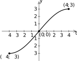
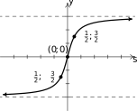
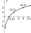
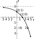
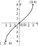
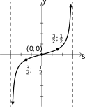
In Section 1.1, we defined functions as processes. In this section, we seek to reverse, or `undo' those processes. As in real life, we will find that some processes (like putting on socks and shoes) are reversible while some (like baking a cake) are not.
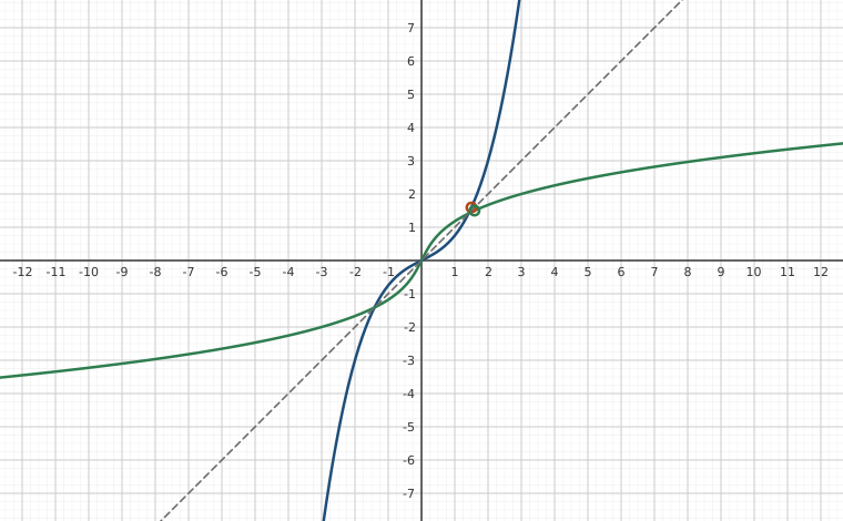
Interactive figureUndoing a function is a reflection: (a, f(a)) becomes (f(a), a)Drag the Input a slider from -3 to 3.
XYZ Graph · viewer build 5edf91b
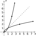
The navy curve is f(x) = x³/4 + x/2, which is always increasing, so every output comes from exactly one input and the process can be undone. Its inverse is drawn in green without ever solving for a formula: the point (f(t), t) is plotted as t runs, which is the definition of the inverse as the same pairs read backwards. Slide a and watch the marker (a, f(a)) on f and its partner (f(a), a) on the inverse move as mirror images across the dashed line y = x, the dashed connector between them always crossing that line at a right angle.
Consider the function . Starting with a real number input , we apply two steps in the following sequence: first we multiply the input by and, second, we add to the result.
To reverse this process, we seek a function which will undo each of these steps and take the output from , , and return the input . If we think of the two-step process of first putting on socks then putting on shoes, to reverse the process, we first take off the shoes and then we take off the socks. In much the same way, the function should undo each step of but in the opposite order. That is, the function should first subtract
from the input then divide the result by . This leads us to the formula .
Let's check to see if the function does the job. If , then . Taking the output from , we substitute it into to get , which is our original input to . To check that does the job for all in the domain of , we take the generic output from , , and substitute that into . That is, we simplify , which is our original input to . If we carefully examine the arithmetic as we simplify , we actually see first `undoing' the addition of , and then `undoing' the multiplication by .
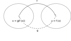
Not only does undo , but also undoes . That is, if we take the output from , , and substitute that into , we get . Using the language of function composition developed in Section 5.3, the statements and can be written as and , respectively.1 Abstractly, we can visualize the relationship between and in the diagram below.
Figure 5.240
The main idea to get from the diagram is that takes the outputs from and returns them to their respective inputs, and conversely, takes outputs from and returns them to their respective inputs. We now have enough background to state the central definition of the section.
If we abstract one step further, we can express the sentiment in Definition 5.4 by saying that and are inverses if and only if and where is the identity function restricted2 to the domain of and is the identity function restricted to the domain of .
In other words, for all in the domain of and for all in the domain of . Using this description of inverses along with the properties of function composition listed in Theorem 5.4, we can show that function inverses are unique.3
Suppose and are both inverses of a function . By Theorem 5.13, the domain of is equal to the domain of , since both are the range of . This means the identity function applies both to the domain of and the domain of . Thus , as required.
We summarize the important properties of invertible functions in the following theorem.4 Apart from introducing notation, each of the results below are immediate consequences of the idea that inverse functions map the outputs from a function back to their corresponding inputs.
The notation is an unfortunate choice since you've been programmed since Elementary Algebra to think of this as . This is most definitely not the case since, for instance, has as its inverse , which is certainly different than .
Why does this confusing notation persist? As we mentioned in Section 5.3, the identity function is to function composition what the real number is to real number multiplication. The choice of notation alludes to the property that and , in much the same way as and .
Before we embark on an example, we demonstrate the pertinent parts of Theorem 5.13 to the inverse pair and . Suppose we wanted to solve . Going through the usual machinations, we obtain .
If we view this equation as , however, then we are looking for the input corresponding to the output . This is exactly the question was built to answer. In other words, the solution to is . In other words, the formula encodes all of the algebra required to `undo' what the formula does to . More generally, any time you have ever solved an equation, you have really been working through an inverse problem.
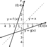
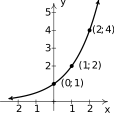
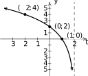
We also note the graphs of and are easily seen to be reflections across the line as seen below. In particular, note that the -intercept on the graph of corresponds to the -intercept on the graph of . Indeed, the point on the graph of can be interpreted as just as the point on the graph of can be interpreted as .
Figure 5.241
Graphs of inverse functions and .
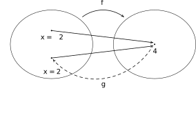
We now investigate under what circumstances a function is invertible. As a way to motivate the discussion, we consider . A likely candidate for the inverse is the function . However, , which is not equal to unless .
For example, when , , but . That is, failed to return the input from its output . Instead, matches the output to a different input, namely , which satisfies . Schematically:
Figure 5.248
We see from the diagram that since both and are , it is impossible to construct a function which takes back to both
and since, by definition, a function can match with only one number.
In general, in order for a function to be invertible, each output can come from only one input. Since, by definition, a function matches up each input to only one output, invertible functions have the property that they match one input to one output and vice-versa. We formalize this concept below.
Note that an equivalent way to state Definition 5.5 is that a function is one-to-one if different inputs go to different outputs. That is, if , then .
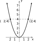
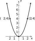
Before we solidify the connection between invertible functions and one-to-one functions, we take a moment to see what goes wrong graphically when trying to find the inverse of .
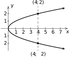
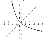
Per Theorem 5.13, the graph of , if it exists, is obtained from the graph of by reflecting about the line . Procedurally, this is accomplished by interchanging the and coordinates of each point on the graph of . Algebraically, we are swapping the variables `' and `' which results in the equation whose graph is below on the right.
Figure 5.249
Figure 5.250
We see immediately the graph of fails the Vertical Line Test, Theorem 1.1. In particular, the vertical line intersects the graph at two points, and meaning the relation described by matches the -value with two different -values, and .
Note that the vertical line and the points on the graph of correspond to the horizontal line and the points on the graph of which brings us right back to the concept of one-to-one. The fact that both and are on the graph of means . Hence, takes different inputs, and , to the same output, , so is not one-to-one.
Recall the Horizontal Line Test from Exercise in Section 1.1. Applying that result to the graph of we say the graph of `fails' the Horizontal Line Test since the horizontal line intersects the graph of more than once. This means that the equation does not represent is not a function of .
Said differently, the Horizontal Line Test detects when there is at least one -value () which is matched to more than one -value (). In other words, the Horizontal Line Test can be used to detect whether or not a function is one-to-one.
So, to review, is not invertible, not one-to-one, and its graph fails the Horizontal Line Test. It turns out that these three attributes: being invertible, one-to-one, and having a graph that passes the Horizontal Line Test are mathematically equivalent. That is to say if one if these things is true about a function, then they all are; it also means that, as in this case, if one of these things isn't true about a function, then none of them are. We summarize this result in the following theorem.
To prove Theorem 5.14, we first suppose is invertible. Then there is a function so that for all in the domain of . If , then . Since , the equation reduces to . We've shown that if , then , proving is one-to-one.
Next, assume is one-to-one. Suppose a horizontal line intersects the graph of at the points and . This means and so . Since is one-to-one, this means so the points and are actually one in the same. This establishes that each horizontal line can intersect the graph of at most once, so the graph of passes the Horizontal Line Test.
Last, but not least, suppose the graph of passes the Horizontal Line Test. Let be a real number in the range of . Then the horizontal line intersects the graph of just once, say at the point . Define the mapping so that . The mapping is a function since each horizontal line where is in the range of intersects the graph of only once. By construction, we have the domain of is the range of and that for all in the domain of ,. We leave it to the reader to show that for all in the domain of , , too.
Hence, we've shown: first, if invertible, then is one-to-one; second, if is one-to-one, then the graph of passes the Horizontal Line Test; and third, if passes the Horizontal Line Test, then is invertible. Hence if is satisfies any one of these three conditions, we can show must satisfy the other two.7
We put this result to work in the next example.
In Example 5.6.2, we showed the functions and are invertible and graphed their inverses. While graphs are perfectly fine representations of functions, we have seen where they aren't the most accurate. Ideally, we would like to represent and in the same manner in which and are presented to us. The key to doing this is to recall that inverse functions take outputs back to their associated inputs.
Consider . As mentioned in Example 5.6.2, the ordered pairs which comprise are in the form . Hence to find a compatible description for , we simply interchange the expressions in each of the coordinates to obtain .
Since the function was defined in terms of a formula we would like to find a formula representation for . We apply the same logic as above. Here, the input, represented by the independent variable , and the output, represented by the dependent variable , are related by the equation . Hence, to exchange inputs and outputs, we interchange the `' and `' variables. Doing so, we obtain the equation which is an implicit description for . Solving for gives an explicit formula for , namely . We demonstrate this technique below.
We claim , and leave the algebraic verification of this to the reader.
We generalize this approach below. As always, we resort to the default `' and `' labels for the independent and dependent variables, respectively.
Steps for finding a formula for the Inverse of a one-to-one function
Write
Interchange and
Solve for to obtain
We now return to . We know that is not one-to-one, and thus, is not invertible, but our goal here is to see what way to see what goes wrong algebraically.
If we attempt to follow the algorithm above to find a formula for , we start with the equation and interchange the variables `' and `' to produce the equation . Solving for gives . It's this `' which is causing the problem for us since this produces two
-values for any .
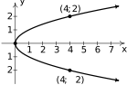
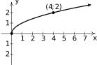
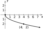
Using the language of Section 5.5, the equation implicitly defines two functions, and , each of which represents the top and bottom halves, respectively, of the graph of .
Figure 5.258Figure 5.259Figure 5.260
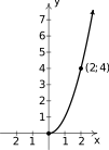
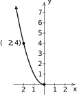
Hence, in some sense, we have two partial inverses for : returns the positive inputs from and returns the negative inputs to . In order to view each of these functions as strict inverses, however, we need to split into two parts: for and for .
Figure 5.261Figure 5.262, Figure 5.263,
We claim that and are an inverse function pair as are and . Indeed, we find:
Figure 5.264, and
Figure 5.265, and
Hence, by restricting the domain of we are able to produce invertible functions. Said differently, in much the same way the equation implicitly describes a pair of functions, the equation implicitly describes a pair of invertible functions.
Our next example continues the theme of restricting the domain of a function to find inverse functions.
Our last example of the section gives an application of inverse functions. Recall in Example 1.2.4 in Section 1.2, we modeled the demand for PortaBoy game systems as the price per system, as a function of the number of systems sold, . In the following example, we find and interpret what it means.
Exercises
In Exercises -, verify the given pairs of functions are inverses algebraically and graphically.
and
and .
and
and
and ,
and , .
and
and , .
In Exercises -, show that the given function is one-to-one and find its inverse. Check your answers algebraically and graphically. Verify the range of the function is the domain of its inverse and vice-versa.
,
,
Explain why each set of ordered pairs below represents a one-to-one function and find the inverse.
In Exercises -, explain why each graph represents12 a one-to-one function and graph its inverse.
Figure 5.270Asymptote: .
Figure 5.271Asymptote: .
Figure 5.272Domain: .
Figure 5.273Asymptotes: .
The price of a dOpi media player, in dollars per dOpi, is given as a function of the weekly sales according to the formula for .
Find and state its domain.
Find and interpret .
The profit (in dollars) made from producing and selling dOpis per week is given by the formula , for . Find and determine what price per dOpi would yield the maximum profit. What is the maximum profit? How many dOpis need to be produced and sold to achieve the maximum profit?
Show that the Fahrenheit to Celsius conversion function found in Exercise in Section 1.2.2 is invertible and that its inverse is the Celsius to Fahrenheit conversion function.
Analytically show that the function is one-to-one. Use Theorem 5.13 to help you compute and . What happens when you attempt to find a formula for ?
Let .
Graph using the techniques in Section 3.2. Check your answer using a graphing utility.
Verify that is one-to-one on the interval .
Use the procedure outlined on Page Section 5.6 to find the formula for for .
Since , it should be the case that . What goes wrong when you attempt to substitute into ? Discuss with your classmates how this problem arose and possible remedies.
With the help of your classmates, explain why a function which is either strictly increasing or strictly decreasing on its entire domain would have to be one-to-one, hence invertible.
If is odd and invertible, prove that is also odd.
Let and be invertible functions. With the help of your classmates show that is one-to-one, hence invertible, and that .
With help from your classmates, find the inverses of the functions in Exercises -.
where .
(See Exercise below.)
What conditions must you place on the values of and in Exercise in order to guarantee that the function is invertible?
The function given in number is an example of a function which is its own inverse.
Algebraically verify every function of the form: is its own inverse.
What assumptions do you need to make about the values of , , and ?
Under what conditions is , its own inverse? Prove your answer.
Answers
,
,
,
,
None of the first coordinates of the ordered pairs in are repeated, so is a function and none of the second coordinates of the ordered pairs of are repeated, so is one-to-one.
Because of the `' it is helpful to determine a formula for the matching. For the even numbers , , the ordered pair is in . For the odd numbers , the ordered pair is in . Hence, given any input to , , whether it be even or odd, there is only one output from , either or , both of which are functions of . To show is one to one, we note that if the output from is or less, then it must be of the form for an even number . Moreover, if , then . In the case we are looking at outputs from which are greater than , then it must be of the form for an odd number . In this, too, if , then . Hence, in any case, if the outputs from are the same, then the inputs to had to be the same so is one-to-one and
To show is a function we note that if we have the same inputs to , say , then . Hence the corresponding outputs, and , are equal, too. To show is one-to-one, we note that if we have the same outputs from , , then . Hence, the corresponding inputs and are equal, too. Hence is one-to-one and
To show is a function, we note that if we have the same inputs to , say , then the outputs from , namely and are equal. To show is one-to-one, we note that if we get the same output from , namely , then . However since and are natural numbers, both and are positive so . Hence is one-to-one and .
. Asymptote: .
Figure 5.274Asymptote: .
. Asymptote: .
Figure 5.275Asymptote: .
. Domain .
Figure 5.276Domain: .
. Asymptotes: .
Figure 5.277Asymptotes: .
. The domain of is the range of which is
. This means that if the price is set to then dOpis will be sold.
, .
The graph of is a parabola opening downwards with vertex . This means that the maximum profit is a whopping when the price per dOpi is set to . At this price, we can produce and sell dOpis. Since we cannot sell part of a system, we need to adjust the price to sell either dOpis or dOpis. We find and , which means we set the price per dOpi at either or , respectively. The profits at these prices are and , so it looks as if the maximum profit is and it is made by producing and selling dOpis a week at a price of per dOpi.
Given that , we have . Similarly and
If , then . If , then and can be any real number.
Adapted from Precalculus with Integrated Calculus, edition 4i, by Carl Stitz and Jeff Zeager (stitz-zeager.com), licensed under CC BY-NC-SA 3.0. Changes were made: reformatted as an accessible XYZ web edition. License: CC-BY-NC-SA-3.0.
These eBooks are a prerelease and are not yet certified conformant with WCAG 2.1 AA or any other accessibility standard. Every page is built against an automated accessibility gate, and our target for the published editions is WCAG 2.2 Level AA. If something is unusable, please tell us.