5.5 Relations and Implicit Functions

Up until now in this text, we have been exclusively special kinds of mappings called functions. In this section, we broaden our horizons to study more general mappings called relations. The reader is encouraged to revisit Definition 1.1 in Section 1.1 before proceeding with the definition of relation below.

Unlike Definition 1.1, Definition 5.3 puts no conditions on the process which maps elements of $A$ to elements of $B$ . This means that while all functions are relations, not all relations need be functions. For example, consider the mappings $f$ and $g$ below from Section 1.1.

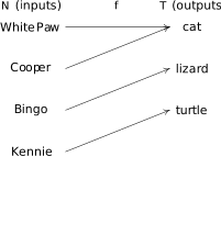
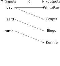
Coordinate-plane figure. — **Figure 5.179**

Both $f$ and $g$ are relations. More specifically, $f$ is a function from $N$ to $T$ while $g$ is merely relation from $T$ to $N$ . As with functions, we may describe general relations in a variety of different ways: verbally, as mapping diagrams, or a set of ordered pairs. For example, just as we may describe the function $f$ above as

$f = {(White Paw, cat), (Cooper, cat), (Bingo, lizard), (Kennie, turtle)},$

we may represent $g$ as

$g = {(cat, White Paw), (cat, Cooper), (lizard, Bingo), (turtle, Kennie)} .$

Note here the grammar ` $g$ is a relation from $T$ to $N$ ' is evidenced by the elements of $T$ being listed first in the ordered pairs (i.e., the abscissae) and the elements of $N$ being listed second (i.e., the ordinates.)

Unlike functions, we do not use function notation when describing the input/output relationship for general relations. For example, we may write ` $f (White Paw) = cat$ ' since $f$ maps the input `White Paw' to only one output, `cat.' However, $g (cat)$ is ambiguous since it could mean `White Paw' or `Cooper.'¹

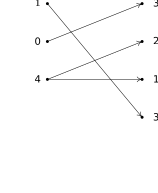
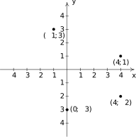
As with functions, our focus in this course will rest with relations of real numbers. Consider the relation $R$ described as follows: $R = {(- 1, 3), (0, - 3), (4, - 2), (4, 1)}$ . Below on the left is a mapping diagram of $R$ . However, since $R$ relates real numbers, we can also create the graph of $R$ in the same way we graphed functions - by interpreting the ordered pairs which comprise $R$ as points in the plane. Since we have no context, we use the default labels ` $x$ ' for the horizontal axis and ` $y$ ' for the vertical axis.

Figure: A Mapping Diagram of . — **Figure 5.181** A Mapping Diagram of $R$ .

Figure: The graph of . — **Figure 5.182** The graph of $R$ .

Our next example focuses on using relations to describe sets of points in the plane and vice-versa.

Example 1

Graph the following relations.
1. $S = {(k, 2^{k}) | k = 0, \pm 1, \pm 2}$
2. $P = {(j, j^{2}) | j is an integer}$
1. $V equals open brace open parenthesis 3, y close parenthesis vertical bar y is a real number close brace$
2. $R equals open brace open parenthesis x, y close parenthesis vertical bar x is a real number, 1 less than y less than or equal to 3 close brace$
Find a roster or set-builder description for each of the relations below.
1. Figure 5.183 The graph of $A$
2. Figure 5.184 The graph of $H$
1. Figure 5.185 The graph of $Q$
2. Figure 5.186 The graph of $T$

1. The relation $S$ is described using set-builder notation.² To generate the ordered pairs which belong to $S$ , we substitute the given values of $k$ , $k = 0, \pm 1, \pm 2$ , into the formula $open parenthesis k, 2 to the power k close parenthesis$ .
  Starting with $k equals 0$ , we get $(0, 2^{0}) = (0, 1)$ . For $k equals 1$ , we get $(1, 2^{1}) = (1, 2)$ , and for $k = - 1$ , we get $(- 1, 2^{- 1}) = (- 1, \frac{1}{2})$ . Continuing, we get $open parenthesis 2, 2 squared close parenthesis equals open parenthesis 2, 4 close parenthesis$ for $k equals 2$ and, finally $(- 2, 2^{- 2}) = (- 2, \frac{1}{4})$ for $k = - 2$ . Hence, a roster description of $S$ is $S = {(- 2, \frac{1}{4}), (- 1, \frac{1}{2}), (0, 1), (1, 2), (2, 4)}$ .
  When we graph $S$ , we label the horizontal axis as the $k$ -axis, since ` $k$ ' was the variable chosen used to generate the ordered pairs and keep the default label ` $y$ ' for the vertical axis. The graph of $S$ is below on the left.
2. To graph the relation $P = {(j, j^{2}) | j is an integer}$ , we proceed as above when we graphed the relation $S$ . Here, $j$ is restricted to being an integer, which means $j equals 0$ , $\pm 1$ , $\pm 2$ , etc.
  Plugging in these sample values for $j$ , we obtain the ordered pairs $open parenthesis 0, 0 close parenthesis$ , $open parenthesis 1, 1 close parenthesis$ , $open parenthesis minus 1, 1 close parenthesis$ , $open parenthesis 2, 4 close parenthesis$ , $open parenthesis minus 2, 4 close parenthesis$ , etc. Since the variable $j$ takes on only integer values, we could write $P$ using the roster notation: $P = {(0, 0), (\pm 1, 1), (\pm 2, 4), \dots}$ .
  We plot a few of these points and use some periods of ellipsis to indicate the complete graph contains additional points not in the current field of view. The graph of $P$ is below on the right.
  Figure 5.187 The graph of $S$
  Figure 5.188 The graph of $P$
3. Next, we come to the relation $V$ , described, once again, using set-builder notation. In this case, $V$ consists of all ordered pairs of the form $open parenthesis 3, y close parenthesis$ where $y$ is free to be whatever real number we like, without any restriction.³ For example, $open parenthesis 3, 0 close parenthesis$ , $open parenthesis 3, minus 1 close parenthesis$ , and $open parenthesis 3, 117 close parenthesis$ all belong to $V$ as do $(3, \frac{1}{2})$ , $open parenthesis 3, minus 1.0342 close parenthesis$ , $open parenthesis 3, the square root of 2 close parenthesis$ , etc.
  After plotting some sample points, becomes apparent that the ordered pairs which belong to $V$ correspond to points which lie on the vertical line $x equals 3$ , and vice-versa. That is, every point on the line $x equals 3$ has coordinates which correspond to an ordered pair belonging to $V$ . The graph of $V$ is below on the left.
4. In the relation $R equals open brace open parenthesis x, y close parenthesis vertical bar 1 less than y less than or equal to 3 close brace$ , we see $y$ is restricted by the inequality $1 less than y less than or equal to 3$ , but $x$ is free to be whatever it likes.
  Since $x$ is unrestricted, this means whatever the graph of $R$ is, it will extend indefinitely off to the right and left. The restriction $y greater than 1$ means all points on the graph of $R$ have a $y$ -coordinate larger than one, so they are above the horizontal line $y equals 1$ . The restriction $y less than or equal to 3$ , on the other hand, means all the points on the graph of $R$ have a $y$ -coordinate less than or equal to $3$ , meaning they are either on or below the horizontal line $y equals 3$ .
  In other words, the graph of $R$ is the region in the plane between $y equals 1$ and $y equals 3$ , including $y equals 3$ but not $y equals 1$ . We signify this by shading the region between these two horizontal lines.
  How do we communicate $y equals 1$ is not part of the graph? One way is to visualize putting `holes' all along the line $y equals 1$ to indicate this is not part of the graph. In practice, however, this looks cluttered and could be confusing. Instead, we `dash' the line $y equals 1$ as seen below on the right.
  Figure 5.189 The graph of $V$
  Figure 5.190 The graph of $R$
1. Since $A$ consists of finitely many points, we can describe $A$ using the roster method:
  $A = {(- 3, 2), (- 3, 1), (0, 0), (4, 2)} .$
2. The graph of $H$ appears to be a portion of the horizontal line $y equals 3$ from $x = - 2$ (including $x = - 2$ ) up to, but not including $x equals 4$ . Since it is impossible⁴ to list each and every one of these points, we'll opt to describe $H$ using set-builder as opposed to the roster method. Taking a cue from the description of the relations $V$ and $R$ above, we write $H = {(x, 3) | - 2 \leq x < 4}$ .
3. The graph of $Q$ appears to be the graph of the function $s = f (t) = t^{2}$ . Again, as the graph consists of infinitely many points, we will use set-builder notation to describe $Q$ out of necessity.
  There are a couple of different ways to do this. Taking a cue from the relation $P$ above, we could write $Q = {(t, t^{2}) | t is a real number}$ . Alternatively, we could introduce the dependent variable, $s$ into the description by writing $Q = {(t, s) | s = t^{2}}$ where here the assumption is $x$ takes in all real number values.
4. As with the relation $R$ above, the relation $T$ describes a region in the plane, The $v$ -values appear to range between $minus 3$ (not including $minus 3$ ) and up to, and including, $v equals 4$ . The only restriction on the $w$ -values is that $w greater than or equal to 1$ , so we have $T = {(v, w) | - 3 < v \leq 4, w \geq 1}$ .

As with functions, we can describe relations algebraically using equations. For example, the equation $v^{2} + w^{3} = 1$ relates two variables $v$ and $w$ each of which represent real numbers. More formally, we can express this sentiment by defining the relation $R = {(v, w) | v^{2} + w^{3} = 1}$ . An ordered pair $open parenthesis v, w close parenthesis ∈ R$ means $v$ and $w$ are related by the equation $v^{2} + w^{3} = 1$ ; that is, the pair $(v, w)$ satisfy the equation.

For example, to show $open parenthesis 3, minus 2 close parenthesis ∈ R$ , we check that when we substitute $v equals 3$ and $w = - 2$ , the equation $v^{2} + w^{3} = 1$ is true. Sure enough, ${(3)}^{2} + {(- 2)}^{3} = 9 - 8 = 1$ . Hence, $R$ maps $3$ to $minus 2$ . Note, however, that $open parenthesis minus 2, 3 close parenthesis ∉ R$ since ${(- 2)}^{2} + {(3)}^{3} = - 8 + 27 \neq 1$ which means $R$ does not map $minus 2$ to $3$ .

When asked to `graph the equation' $v^{2} + w^{3} = 1$ , we really have two options. We could graph the relation $R$ above. In this case, we would be graphing $v^{2} + w^{3} = 1$ on the $v w$ -plane.⁵ Alternatively, we could define $S = {(w, v) | v^{2} + w^{3} = 1}$ and graph $S$ . This is equivalent to graphing $v^{2} + w^{3} = 1$ on the $w v$ -plane. We do both in our next example.

Example 2

Graph the equation $v^{2} + w^{3} = 1$ in the $v w$ - and $w v$ -planes. Include the axis-intercepts.

graphing in the $v w$ -plane: We begin by finding the axis intercepts of the graph. To obtain a point on the $v$ -axis, we require $w equals 0$ . To see if we have any $v$ -intercepts on the graph of the equation $v^{2} + w^{3} = 1$ , we substitute $w equals 0$ into the equation and solve for $v$ : $v^{2} + {(0)}^{3} = 1$ . We get $v squared equals 1$ or $v = \pm 1$ so our two $v$ -intercepts, as described in the $v w$ -plane, are $open parenthesis 1, 0 close parenthesis$ and $open parenthesis minus 1, 0 close parenthesis$ .
Likewise, to find $w$ -intercepts of the graph, we substitute $v equals 0$ into the equation $v^{2} + w^{3} = 1$ and get $w cubed equals 1$ or $w equals 1$ . Hence, he have only one $w$ -intercept, $open parenthesis 0, 1 close parenthesis$ .
One way to efficiently produce additional points is to solve the equation $v^{2} + w^{3} = 1$ for one of the variables, say $w$ , in terms of the other, $v$ . In this way, we are treating $w$ as the dependent variable and $v$ as the independent variable. From $v^{2} + w^{3} = 1$ , we get $w^{3} = 1 - v^{2}$ or $w = \sqrt[3]{1 - v^{2}}$ .
We now substitute a value in for $v$ , determine the corresponding value $w$ , and plot the resulting point $(v, w)$ . We summarize our results below on the left. By plotting additional points (or getting help from a graphing utility), we produce the graph below on the right.
$\begin{matrix} v & w & (v, w) \\ - 3 & - 2 & (- 3, - 2) \\ - 2 & - \sqrt[3]{3} & (- 2, - \sqrt[3]{3}) \\ - 1 & 0 & (- 1, 0) \\ 0 & 1 & (0, 1) \\ 1 & 0 & (1, 0) \\ 2 & - \sqrt[3]{3} & (2, - \sqrt[3]{3}) \\ 3 & - 2 & (3, - 2) \end{matrix}$
Figure 5.191 $v^{2} + w^{3} = 1$
graphing in the $w v$ -plane: To graph $v^{2} + w^{3} = 1$ in the $w v$ -plane, all we need to do is reverse the coordinates of the ordered pairs we obtained for our graph in the $v w$ -plane. In particular, the $v$ -intercepts are written $open parenthesis 0, 1 close parenthesis$ and $open parenthesis 0, minus 1 close parenthesis$ and the $w$ -intercept is written $open parenthesis 1, 0 close parenthesis$ . Using the table below on the left we produce the graph below on the right.
$\begin{matrix} v & w & (w, v) \\ - 3 & - 2 & (- 2, - 3) \\ - 2 & - \sqrt[3]{3} & (- \sqrt[3]{3}, - 2) \\ - 1 & 0 & (0, - 1) \\ 0 & 1 & (1, 0) \\ 1 & 0 & (0, 1) \\ 2 & - \sqrt[3]{3} & (- \sqrt[3]{3}, 2) \\ 3 & - 2 & (- 2, 3) \end{matrix}$
Figure 5.192 $v^{2} + w^{3} = 1$

Note that regardless of which geometric depiction we choose for $v^{2} + w^{3} = 1$ , the graph appears to be symmetric about the $w$ -axis. To prove this is the case, consider a generic point $(v, w)$ on the graph of $v^{2} + w^{3} = 1$ in the $v w$ -plane.

To show the point symmetric about the $w$ -axis, $(- v, w)$ is also on the graph of $v^{2} + w^{3} = 1$ , we need to show that the coordinates of the point $(- v, w)$ satisfy the equation $v^{2} + w^{3} = 1$ . That is, we need to show ${(- v)}^{2} + w^{3} = 1$ . Since ${(- v)}^{2} + w^{3} = v^{2} + w^{3}$ , and we know by assumption $v^{2} + w^{3} = 1$ , we get ${(- v)}^{2} + w^{3} = v^{2} + w^{3} = 1$ , proving $(- v, w)$ is also on the graph of the equation.

The key reason our proof above is successful is that algebraically, the equation $v^{2} + w^{3} = 1$ is unchanged if $v$ is replaced with $- v$ . Geometrically, this means the graph is the same if it undergoes a reflection across the $w$ -axis. We generalize this reasoning in the following result. Note that, as usual, we default to the more common $x$ and $y$ -axis labels.

Theorem

Testing the Graph of an Equation for Symmetry:

To test the graph of an equation in the $x y$ -plane for symmetry:

about the $x$ -axis: substitute $(x, - y)$ into the equation and simplify. If the result is equivalent to the original equation, the graph is symmetric about the $x$ -axis.
about the $y$ -axis: substitute $(- x, y)$ into the equation and simplify. If the result is equivalent to the original equation, the graph is symmetric about the $y$ -axis.
about the origin: substitute $(- x, - y)$ into the equation and simplify. If the result is equivalent to the original equation, the graph is symmetric about the origin.

Parts of Theorem 5.12 should look familiar from our work with even and odd functions. Indeed if a function $f$ is even, $f (- x) = f (x)$ . Hence, the equation $y = f (- x)$ reduces to the equation $y = f (x)$ , so the graph of $f$ is symmetric about the $y$ -axis.

Likewise if $f$ is odd, then $f (- x) = - f (x)$ . In this case, the equation $- y = f (- x)$ reduces to $- y = - f (x)$ , or $y = f (x)$ , proving the graph is symmetric about the origin.

When it comes to symmetry about the $x$ -axis, most of the time this indicates a violation of the Vertical Line Test, which is why we haven't discussed that particular kind of symmetry until now.

We put Theorem 5.12 to good use in the following example.

Example 3

Graph each of the equations below in the $x y$ -plane. Find the axis intercepts, if any, and prove any symmetry suggested by the graphs.

$x^{2} - y^{2} = 4$
${(x - 1)}^{2} + 4 y^{2} = 16$

We begin graphing $x^{2} - y^{2} = 4$ by checking for axis intercepts. To check for $x$ -intercepts, we set $y equals 0$ and solve $x^{2} - {(0)}^{2} = 4$ . We get $x = \pm 2$ and obtain two $x$ -intercepts $open parenthesis minus 2, 0 close parenthesis$ and $open parenthesis 2, 0 close parenthesis$ .
When looking for $y$ -intercepts, we set $x equals 0$ and get ${(0)}^{2} - y^{2} = 4$ or $y^{2} = - 4$ . Since this equation has no real number solutions, we have no $y$ -intercepts.
In order to produce more points on the graph, we solve $x^{2} - y^{2} = 4$ for $y$ and obtain $y = \pm \sqrt{x^{2} - 4}$ . Since we know $x squared minus 4 greater than or equal to 0$ in order to produce real number results for $y$ , we restrict our attention to $x less than or equal to minus 2$ and $x greater than or equal to 2$ . Doing so produces the table below on the left. Using these, we construct the graph below the right.
The graph certainly appears to be symmetric about both axes and the origin. To prove this, we note that the equation $x^{2} - {(- y)}^{2} = 4$ quickly reduces to $x^{2} - y^{2} = 4$ , proving the graph is symmetric about the $x$ -axis.
Likewise, the equations ${(- x)}^{2} - y^{2} = 4$ and ${(- x)}^{2} - {(- y)}^{2} = 4$ also reduce to $x^{2} - y^{2} = 4$ , proving the graph is, indeed, symmetric about the $y$ -axis and origin, respectively.
$\begin{matrix} x & y & (x, y) \\ - 4 & \pm 2 \sqrt{3} & (- 4, \pm 2 \sqrt{3}) \\ - 3 & \pm \sqrt{5} & (- 3, \pm \sqrt{5}) \\ - 2 & 0 & (- 2, 0) \\ 2 & 0 & (2, 0) \\ 3 & \pm \sqrt{5} & (3, \pm \sqrt{5}) \\ 4 & \pm 2 \sqrt{3} & (4, \pm 2 \sqrt{3}) \end{matrix}$
Figure 5.193 $x^{2} - y^{2} = 4$
To determine if there are any $x$ -intercepts on the graph of ${(x - 1)}^{2} + 4 y^{2} = 16$ , we set $y equals 0$ and solve ${(x - 1)}^{2} + 4 {(0)}^{2} = 16$ . This reduces to ${(x - 1)}^{2} = 16$ which gives $x = - 3$ and $x equals 5$ . Hence, we have two $x$ -intercepts, $open parenthesis minus 3, 0 close parenthesis$ and $open parenthesis 5, 0 close parenthesis$ .
Looking for $y$ -intercepts, we set $x equals 0$ and solve ${(0 - 1)}^{2} + 4 y^{2} = 16$ or $1 + 4 y^{2} = 16$ . This gives $y^{2} = \frac{15}{4}$ so $y = \pm \frac{\sqrt{15}}{2}$ . Hence, we have two $y$ -intercepts: $(0, \pm \frac{\sqrt{15}}{2})$ .
In this case, it is slightly easier⁶ to solve for $x$ in terms of $y$ . From ${(x - 1)}^{2} + 4 y^{2} = 16$ we get ${(x - 1)}^{2} = 16 - 4 y^{2}$ which gives $x = 1 \pm \sqrt{16 - 4 y^{2}}$ .
Since we know $16 minus 4 ⁢ y squared greater than or equal to 0$ to produce real number results for $x$ , we require $minus 2 less than or equal to y less than or equal to 2$ . Selecting values in that range produces the table below on the left. Plotting these points, along with the $y$ -intercepts produces the graph on the right.
$\begin{matrix} y & x & (x, y) \\ - 2 & 1 & (1, - 2) \\ - 1 & 1 \pm 2 \sqrt{3} & (1 \pm 2 \sqrt{3}, - 1) \\ 0 & 1 \pm 4 = - 3, 5 & (- 3, 0), (5, 0) \\ 1 & 1 \pm 2 \sqrt{3} & (1 \pm 2 \sqrt{3}, 1) \\ 2 & 1 & (1, 2) \end{matrix}$
Figure 5.194 ${(x - 1)}^{2} + 4 y^{2} = 16$
The graph certainly appears to be symmetric about the $x$ -axis. To check, we substitute $(- y)$ in for $y$ and get ${(x - 1)}^{2} + 4 {(- y)}^{2} = 16$ which reduces to ${(x - 1)}^{2} + 4 y^{2} = 16$ .
Owing to the placement of the $x$ -intercepts, $open parenthesis minus 3, 0 close parenthesis$ and $open parenthesis 5, 0 close parenthesis$ , the graph is most certainly not symmetric about the $y$ -axis nor about the origin.

Looking at the graphs of the equations $x^{2} - y^{2} = 4$ and ${(x - 1)}^{2} + 4 y^{2} = 16$ in Example 5.5.3, it is evident neither of these equations represents $y$ as a function of $x$ nor $x$ as a function of $y$ . (Do you see why?)

With the concept of `function' being touted in the opening remarks of Section 1.1 as being one of the `universal tools' with which scientists and engineers solve a wide variety of problems, you may well wonder if we can't somehow apply what we know about functions to these sorts of relations. It turns out that while, taken all at once, these equations do not describe functions, taken in parts, they do.

For example, consider the equation $x^{2} - y^{2} = 4$ . Solving for $y$ , we obtained $y = \pm \sqrt{x^{2} - 4}$ . Defining $f_{1} (x) = \sqrt{x^{2} - 4}$ and $f_{2} (x) = - \sqrt{x^{2} - 4}$ , we get a functional description for the upper and lower halves, or branches of the curve, respectively.⁷

If, for instance, we wanted to analyze this curve near $(3, - \sqrt{5})$ , we could use the function $f sub 2$ and all the associated function tools⁸ to do just that.

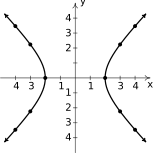
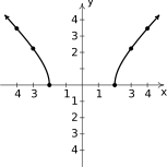
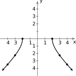
In this way we say the equation $x^{2} - y^{2} = 4$ implicitly describes $y$ as a function of $x$ meaning that given any point $open parenthesis x sub 0, y sub 0 close parenthesis$ on $x^{2} - y^{2} = 4$ , we can find a function $f$ defined (on an interval) containing $x sub 0$ so that $f ⁢ open parenthesis x sub 0 close parenthesis equals y sub 0$ and whose graph lies on the curve $x^{2} - y^{2} = 4$ .

Note that in this case, we are fortunate to have two explicit formulas for functions that cover the entire curve, namely $f_{1} (x) = \sqrt{x^{2} - 4}$ and $f_{2} (x) = - \sqrt{x^{2} - 4}$ . We explore this concept further in the next example.

Example 4

Consider the graph of the relation $R$ below.

Explain why this curve does not represent $y$ as a function of $x$ .
Resolve the graph of $R$ into two or more graphs of implicitly defined functions.
Explain why this curve represents $x$ as a function of $y$ and find a formula for $x = g (y)$ .

Figure 5.198 The graph of

R

Using the Vertical Line Test, Theorem 1.1, we find several instances where vertical lines intersect the graph of $R$ more than once. The $y$ -axis, $x equals 0$ is one such line. We have $x equals 0$ matched with three different $y$ -values: $- \sqrt{3}$ , $0$ , and $the square root of 3$ .
Since the maximum number of times a vertical line intersects the graph of $R$ is three, it stands to reason we need to resolve the graph of $R$ into at least three pieces.
One strategy is to begin at the far left and begin tracing the graph until it begins to `double back' and repeat $y$ -coordinates. Doing so we get three functions (represented by the bold solid lines) below.
Figure 5.199 $y equals f sub 1 ⁢ open parenthesis x close parenthesis$
Figure 5.200 $y equals f sub 2 ⁢ open parenthesis x close parenthesis$
Figure 5.201 $y equals f sub 3 ⁢ open parenthesis x close parenthesis$
To verify that $R$ represents $x$ as a function of $y$ , we check to see if any $y$ -value has more than one $x$ associated with it. One way to do this is to employ the the Horizontal Line Test (Exercise in Section 1.1.) Since every horizontal line intersects the graph at most once, $x$ is a function of $y$ .
Using Theorem 2.16 from Chapter 2, we get $x = (1) y (y - \sqrt{3}) (y + \sqrt{3}) = y^{3} - 3 y$ , a fact we can readily check using a graphing utility.

Not all equations implicitly define $y$ as a function of $x$ . For a quick example, take $x equals 117$ or any other vertical line. Even if an equation implicitly describes $y$ as a function of $x$ near one point, there's no guarantee we can find an explicit algebraic representation for that function.⁹

While the theory of implicit functions is well beyond the scope of this text, we will nevertheless see this concept come into play in Section 5.6. For our purposes, it suffices to know that just because a relation is not a function doesn't mean we cannot find a way to apply what we know about functions to analyze the relation locally through a functional lens.

Exercises

In Exercises -, graph the given relation in the $x y$ -plane.

{ $open parenthesis minus 3, 9 close parenthesis$ , $open parenthesis minus 2, 4 close parenthesis$ , $open parenthesis minus 1, 1 close parenthesis$ , $open parenthesis 0, 0 close parenthesis$ , $open parenthesis 1, 1 close parenthesis$ , $open parenthesis 2, 4 close parenthesis$ , $open parenthesis 3, 9 close parenthesis close brace$
{ $open parenthesis minus 2, 0 close parenthesis$ , $open parenthesis minus 1, 1 close parenthesis$ , $(- 1, - 1)$ , $open parenthesis 0, 2 close parenthesis$ , $open parenthesis 0, minus 2 close parenthesis$ , $open parenthesis 1, 3 close parenthesis$ , $open parenthesis 1, minus 3 close parenthesis close brace$
${(m, 2 m) | m = 0, \pm 1, \pm 2}$
${(\frac{6}{k}, k) | k = \pm 1, \pm 2, \pm 3, \pm 4, \pm 5, \pm 6}$
${(n, 4 - n^{2}) | n = 0, \pm 1, \pm 2}$
${(\sqrt{j}, j) | j = 0, 1, 4, 9}$
${(x, - 2) | x > - 4}$
$open brace open parenthesis x, 3 close parenthesis vertical bar x less than or equal to 4 close brace$
$open brace open parenthesis minus 1, y close parenthesis vertical bar y greater than 1 close brace$
$open brace open parenthesis 2, y close parenthesis vertical bar y less than or equal to 5 close brace$
${(- 2, y) | - 3 < y \leq 4}$
$open brace open parenthesis 3, y close parenthesis vertical bar minus 4 less than or equal to y less than 3 close brace$
$open brace open parenthesis x, 2 close parenthesis vertical bar minus 2 less than or equal to x less than 3 close brace$
${(x, - 3) | - 4 < x \leq 4}$
$open brace open parenthesis x, y close parenthesis vertical bar x greater than minus 2 close brace$
$open brace open parenthesis x, y close parenthesis vertical bar x less than or equal to 3 close brace$
$open brace open parenthesis x, y close parenthesis vertical bar y less than 4 close brace$
$open brace open parenthesis x, y close parenthesis vertical bar x less than or equal to 3, y less than 2 close brace$
$open brace open parenthesis x, y close parenthesis vertical bar x greater than 0, y less than 4 close brace$
${(x, y) | - \sqrt{2} \leq x \leq \frac{2}{3}, π < y \leq \frac{9}{2}}$

In Exercises -, describe the given relation using either the roster or set-builder method.

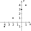
Figure 5.202 Relation 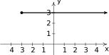$A$
Figure 5.203 Relation 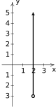$B$
Figure 5.204 Relation 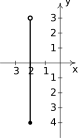$C$
Figure 5.205 Relation 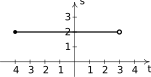$D$
Figure 5.206 Relation 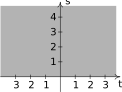$E$
Figure 5.207 Relation 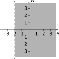$F$
Figure 5.208 Relation 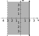$G$
Figure 5.209 Relation 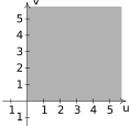$H$
Figure 5.210 Relation 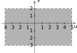$I$
Figure 5.211 Relation $J$

Some relations are fairly easy to describe in words or with the roster method but are rather difficult, if not impossible, to graph. Discuss with your classmates how you might graph the relations given in Exercises -. Note that in the notation below we are using the ellipsis, `…,' to denote that the list does not end, but rather, continues to follow the established pattern indefinitely.

For the relations in Exercises and, give two examples of points which belong to the relation and two points which do not belong to the relation.

${(x, y) | x is an odd integer, and y is an even integer.}$
$open brace open parenthesis x, 1 close parenthesis vertical bar x ⁢ is an irrational number close brace$
$open brace open parenthesis 1, 0 close parenthesis, open parenthesis 2, 1 close parenthesis, open parenthesis 4, 2 close parenthesis, open parenthesis 8, 3 close parenthesis, open parenthesis 16, 4 close parenthesis, open parenthesis 32, 5 close parenthesis, … close brace$
${\dots, (- 3, 9), (- 2, 4), (- 1, 1), (0, 0), (1, 1), (2, 4), (3, 9), \dots}$

For each equation given in Exercises -:

Graph the equation in the $x y$ -plane by creating a table of points.
Find the axis intercepts, if they exist.
Test the equation for symmetry. If the equation fails a symmetry test, find a point on the graph of the equation whose symmetric point is not on the graph of the equation.
Determine if the equation describes $y$ as a function of $x$ . If not, describe the graph of the equation using two or more explicit functions of $x$ . Check your answers using a graphing utility.
${(x + 2)}^{2} + y^{2} = 16$
$x^{2} - y^{2} = 1$
$4 y^{2} - 9 x^{2} = 36$
$x^{3} y = - 4$

For each equation given in Exercises -:

Graph the equation in the $v w$ -plane by creating a table of points.
Find the axis intercepts, if they exist.
Test the equation for symmetry. If the equation fails a symmetry test, find a point on the graph of the equation whose symmetric point is not on the graph of the equation.
Determine if the equation describes $w$ as a function of $v$ . If not, describe the graph of the equation using two or more explicit functions of $v$ . Check your answers using a graphing utility.
$v + w^{2} = 4$
$v^{3} + w^{3} = 8$
$v squared ⁢ w cubed equals 8$
¹⁰ $v^{4} - 2 v^{2} w + w^{2} = 16$

The procedures which we have outlined in the Examples of this section and used in Exercises - all rely on the fact that the equations were “well-behaved”. Not everything in Mathematics is quite so tame, as the following equations will show you. Discuss with your classmates how you might approach graphing the equations given in Exercises -. What difficulties arise when trying to apply the various tests and procedures given in this section? For more information, including pictures of the curves, each curve name is a link to its page at www.wikipedia.org. For a much longer list of fascinating curves, click here .

$x^{3} + y^{3} - 3 x y = 0$ Folium of Descartes
$x^{4} = x^{2} + y^{2}$ Kampyle of Eudoxus
$y^{2} = x^{3} + 3 x^{2}$ Tschirnhausen cubic
${(x^{2} + y^{2})}^{2} = x^{3} + y^{3}$ Crooked egg
With the help of your classmates, find examples of equations whose graphs possess
- symmetry about the $x$ -axis only
- symmetry about the $y$ -axis only
- symmetry about the origin only
- symmetry about the $x$ -axis, $y$ -axis, and origin
Can you find an example of an equation whose graph possesses exactly two of the symmetries listed above? Why or why not?

Answers

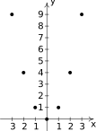
Figure 5.212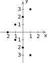
Figure 5.213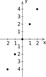
Figure 5.214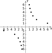
Figure 5.215
Figure 5.216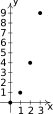
Figure 5.217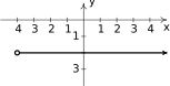
Figure 5.218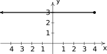
Figure 5.219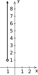
Figure 5.220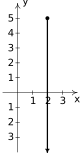
Figure 5.221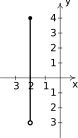
Figure 5.222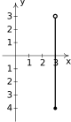
Figure 5.223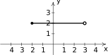
Figure 5.224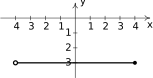
Figure 5.225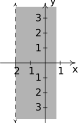
Figure 5.226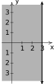
Figure 5.227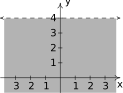
Figure 5.228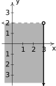
Figure 5.229
Figure 5.230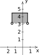
Figure 5.231
$A = {(- 4, - 1), (- 2, 1), (0, 3), (1, 4)}$
$B = {(x, 3) | x \geq - 3}$
$C = {(2, y) | y > - 3}$
$D = {(- 2, y) | - 4 \leq y < 3}$
$E = {(t, 2) | - 4 < t \leq 3}$
$F equals open brace open parenthesis t, s close parenthesis vertical bar s greater than or equal to 0 close brace$
$G = {(v, w) | v > - 2}$
$H = {(v, w) | - 3 < v \leq 2}$
$I equals open brace open parenthesis u, v close parenthesis vertical bar u greater than or equal to 0, v greater than or equal to 0 close brace$
$J = {(u, v) | - 4 < u < 5, - 3 < v < 2}$
${(x + 2)}^{2} + y^{2} = 16$ Re-write as $y = \pm \sqrt{16 - {(x + 2)}^{2}}$ .
$x$ -intercepts: $open parenthesis minus 6, 0 close parenthesis$ , $open parenthesis 2, 0 close parenthesis$
$y$ -intercepts: $(0, \pm 2 \sqrt{3})$
$\begin{matrix} x & y & (x, y) \\ - 6 & 0 & (- 6, 0) \\ - 4 & \pm 2 \sqrt{3} & (- 4, \pm 2 \sqrt{3}) \\ - 2 & \pm 4 & (- 2, \pm 4) \\ 0 & \pm 2 \sqrt{3} & (0, \pm 2 \sqrt{3}) \\ 2 & 0 & (2, 0) \end{matrix}$
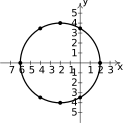
Figure 5.232
The graph is symmetric about the $x$ -axis
The graph is not symmetric about the $y$ -axis: $open parenthesis minus 6, 0 close parenthesis$ is on the graph but $open parenthesis 6, 0 close parenthesis$ is not.
The graph is not symmetric about the origin: $open parenthesis minus 6, 0 close parenthesis$ is on the graph but $open parenthesis 6, 0 close parenthesis$ is not.
The equation does not describe $y$ as a function of $x$ .
The graph of the equation is the graphs of $f_{1} (x) = \sqrt{16 - {(x + 2)}^{2}}$ together with $f_{2} (x) = - \sqrt{16 - {(x + 2)}^{2}}$ .
$x^{2} - y^{2} = 1$ Re-write as: $y = \pm \sqrt{x^{2} - 1}$ .
$x$ -intercepts: $open parenthesis minus 1, 0 close parenthesis, open parenthesis 1, 0 close parenthesis$
The graph has no $y$ -intercepts
$\begin{matrix} x & y & (x, y) \\ - 3 & \pm \sqrt{8} & (- 3, \pm \sqrt{8}) \\ - 2 & \pm \sqrt{3} & (- 2, \pm \sqrt{3}) \\ - 1 & 0 & (- 1, 0) \\ 1 & 0 & (1, 0) \\ 2 & \pm \sqrt{3} & (2, \pm \sqrt{3}) \\ 3 & \pm \sqrt{8} & (3, \pm \sqrt{8}) \end{matrix}$
Figure 5.233
The graph is symmetric about the $x$ -axis.
The graph is symmetric about the $y$ -axis.
The graph is symmetric about the origin.
The equation does not describe $y$ as a function of $x$ .
The graph of the equation is the graphs of $f_{1} (x) = \sqrt{x^{2} - 1}$ together with $f_{2} (x) = - \sqrt{x^{2} - 1}$ .
$4 y^{2} - 9 x^{2} = 36$
Re-write as: $y = \pm \frac{\sqrt{9 x^{2} + 36}}{2}$ .
The graph has no $x$ -intercepts
$y$ -intercepts: $(0, \pm 3)$
$\begin{matrix} x & y & (x, y) \\ - 4 & \pm 3 \sqrt{5} & (- 4, \pm 3 \sqrt{5}) \\ - 2 & \pm 3 \sqrt{2} & (- 2, \pm 3 \sqrt{2}) \\ 0 & \pm 3 & (0, \pm 3) \\ 2 & \pm 3 \sqrt{2} & (2, \pm 3 \sqrt{2}) \\ 4 & \pm 3 \sqrt{5} & (4, \pm 3 \sqrt{5}) \end{matrix}$
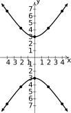
Figure 5.234
The graph is symmetric about the $x$ -axis.
The graph is symmetric about the $y$ -axis.
The graph is symmetric about the origin.
The equation does not describe $y$ as a function of $x$ .
The graph of the equation is the graphs of $f_{1} (x) = \frac{\sqrt{9 x^{2} + 36}}{2}$ together with $f_{2} (x) = - \frac{\sqrt{9 x^{2} + 36}}{2}$ .
$x^{3} y = - 4$ Re-write as: $y = - \frac{4}{x^{3}} = - 4 x^{- 3}$ .
The graph has no $x$ -intercepts
The graph has no $y$ -intercepts
$\begin{matrix} x & y & (x, y) \\ - 2 & \frac{1}{2} & (- 2, \frac{1}{2}) \\ - 1 & 4 & (- 1, 4) \\ - \frac{1}{2} & 32 & (- \frac{1}{2}, 32) \\ \frac{1}{2} & - 32 & (\frac{1}{2}, - 32) \\ 1 & - 4 & (1, - 4) \\ 2 & - \frac{1}{2} & (2, - \frac{1}{2}) \end{matrix}$
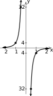
Figure 5.235
The graph is not symmetric about the $x$ -axis: $open parenthesis 1, minus 4 close parenthesis$ is on the graph but $open parenthesis 1, 4 close parenthesis$ is not.
The graph is not symmetric about the $y$ -axis: $open parenthesis 1, minus 4 close parenthesis$ is on the graph but $(- 1, - 4)$ is not.
The graph is symmetric about the origin.
The equation does describe $y$ as a function of $x$ , namely $y = f (x) = - 4 x^{- 3}$ .
$v + w^{2} = 4$ Re-write as $w = \pm \sqrt{4 - v}$ .
$v$ -intercept: $open parenthesis 4, 0 close parenthesis$
$w$ -intercepts: $(0, \pm 2)$
$\begin{matrix} v & w & (x, y) \\ - 5 & \pm 3 & (- 5, \pm 3) \\ - 2 & \pm \sqrt{6} & (- 2, \pm \sqrt{6}) \\ 0 & \pm 2 & (0, \pm 2) \\ 2 & \pm \sqrt{2} & (1, \pm \sqrt{3}) \\ 4 & 0 & (4, 0) \end{matrix}$
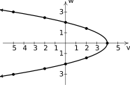
Figure 5.236
The graph is symmetric about the $v$ -axis
The graph is not symmetric about the $w$ -axis: $open parenthesis 4, 0 close parenthesis$ is on the graph but $open parenthesis minus 4, 0 close parenthesis$ is not.
The graph is not symmetric about the origin: $open parenthesis 4, 0 close parenthesis$ is on the graph but $open parenthesis minus 4, 0 close parenthesis$ is not.
The equation does not describe $w$ as a function of $v$ .
The graph of the equation is the graphs of $f_{1} (v) = \sqrt{4 - v}$ together with $f_{2} (v) = - \sqrt{4 - v}$ .
$v^{3} + w^{3} = 8$ Re-write as: $w = \sqrt[3]{8 - v^{3}}$ .
$v$ -intercept: $open parenthesis 2, 0 close parenthesis$
$w$ -intercept: $open parenthesis 0, 2 close parenthesis$
$\begin{matrix} v & w & (v, w) \\ - 3 & \sqrt[3]{35} & (- 3, \sqrt[3]{35}) \\ - 1 & \sqrt[3]{9} & (- 1, \sqrt[3]{9}) \\ 0 & 2 & (0, 2) \\ 1 & \sqrt[3]{7} & (1, \sqrt[3]{7}) \\ 2 & 0 & (2, 0) \\ 3 & - \sqrt[3]{19} & (3, - \sqrt[3]{19}) \end{matrix}$
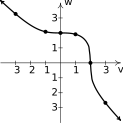
Figure 5.237
The graph is not symmetric about the $v$ -axis: $open parenthesis 0, 2 close parenthesis$ is on the graph but $open parenthesis 0, minus 2 close parenthesis$ is not.
The graph is not symmetric about the $w$ -axis: $open parenthesis 2, 0 close parenthesis$ is on the graph but $open parenthesis minus 2, 0 close parenthesis$ is not.
The graph is not symmetric about the origin: $open parenthesis 0, 2 close parenthesis$ is on the graph but $open parenthesis 0, minus 2 close parenthesis$ is not.
The equation does describe $w$ as a function of $v$ , namely $w = f (v) = \sqrt[3]{8 - v^{3}}$ .
$v squared ⁢ w cubed equals 8$ Re-write as $w = \frac{2}{\sqrt[3]{v^{2}}} = 2 v^{- \frac{2}{3}}$ .
The graph has no $v$ -intercepts.
The graph has no $w$ -intercepts.
$\begin{matrix} v & w & (x, y) \\ - 8 & \frac{1}{2} & (- 8, \frac{1}{2}) \\ - 1 & 2 & (- 1, 2) \\ - \frac{1}{8} & 8 & (- \frac{1}{8}, 8) \\ \frac{1}{8} & 8 & (\frac{1}{8}, 8) \\ 1 & 2 & (1, 2) \\ 8 & \frac{1}{2} & (8, \frac{1}{2}) \end{matrix}$
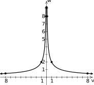
Figure 5.238
The graph is not symmetric about the $v$ -axis: $open parenthesis minus 1, 2 close parenthesis$ is on the graph but $(- 1, - 2)$ is not.
The graph is symmetric about the $w$ -axis.
The graph is not symmetric about the origin: $open parenthesis minus 1, 2 close parenthesis$ is on the graph but $(- 1, - 2)$ is not.
The equation does describe $w$ as a function of $v$ , namely $w = f (v) = 2 v^{- \frac{2}{3}}$ .
$v^{4} - 2 v^{2} w + w^{2} = 16$ Re-write as: ${(v^{2} - w)}^{2} = 16$ Extracting square roots gives: $w = v^{2} + 4$ and $w = v^{2} - 4$
$v$ -intercepts: $open parenthesis minus 2, 0 close parenthesis, open parenthesis 2, 0 close parenthesis$ .
$w$ -intercepts: $open parenthesis 0, minus 4 close parenthesis, open parenthesis 0, 4 close parenthesis$
$\begin{matrix} v & w & (v, w) \\ - 2 & 8 & (- 2, 8) \\ - 2 & 0 & (- 2, 0) \\ - 1 & 5 & (- 1, 5) \\ - 1 & - 3 & (- 1, - 3) \\ 0 & \pm 4 & (0, \pm 4) \\ 1 & 5 & (1, 5) \\ 1 & - 3 & (1, - 3) \\ 2 & 8 & (2, 8) \\ 2 & 0 & (2, 0) \end{matrix}$
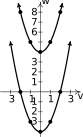
Figure 5.239
The graph is not symmetric about the $v$ -axis: $open parenthesis 1, 5 close parenthesis$ is on the graph but $open parenthesis 1, minus 5 close parenthesis$ is not.
The graph is symmetric about the $w$ -axis.
The graph is not symmetric about the origin: $open parenthesis 1, 5 close parenthesis$ is on the graph but $(- 1, - 5)$ is not.
The equation does not describe $w$ as a function of $v$ .
The graph of the equation is the graphs of $f_{1} (v) = v^{2} + 4$ together with $f_{2} (v) = v^{2} - 4$ .

In more advanced texts, we would write ` $cat g White Paw$ ' and ` $cat g Cooper$ ' to indicate $g$ maps `cat' to both `White Paw' and `Cooper.' Our study of relations, however, isn't deep enough to necessitate introducing and using this notation. Similarly, we won't introduce the notions of `domain,' `codomain,' and `range' for relations, either. ↩
See Section A.1 to review this, if needed. ↩
We'll revisit the concept of a `free variable' in Section 9.1. ↩
Really impossible. The interested reader is encouraged to research countable versus uncountable sets. ↩
Recall this means the horizontal axis is labeled ` $v$ ' and the vertical axis is labeled ` $w$ .' ↩
Read this as we're avoiding fractions. ↩
There are many more ways to break this relation into functional parts. We could, for instance, go piecewise and take portions of the graph which lie in Quadrants I and III as one function and leave the parts in Quadrants II and IV as the other; we could look at this as being comprised of four functions, and so on. ↩
including, when the time comes, Calculus ↩
An example of this is $y^{5} - y - x = 1$ near $open parenthesis minus 1, 0 close parenthesis$ . ↩
HINT: $v^{4} - 2 v^{2} w + w^{2} = {(v^{2} - w)}^{2}$ … ↩

Adapted from Precalculus, Preliminary 4th Edition (integrated calculus), by Carl Stitz and Jeff Zeager (stitz-zeager.com), licensed under CC BY-NC-SA 3.0. Changes were made: reformatted as an accessible XYZ web edition. License: CC-BY-NC-SA-3.0.