As we mentioned in Section 5.1, in this chapter, we are studying functions in a more abstract and general setting. In this section, we begin our study of what can be considered as the algebra of functions by defining function arithmetic.
Given two real numbers, we have four primary arithmetic operations available to us: addition, subtraction, multiplication, and division (provided we don't divide by .) Since the functions we study in this text have ranges which are sets of real numbers, it makes sense we can extend these arithmetic notions to functions.
For example, to add two functions means we add their outputs; to subtract two functions, we subtract their outputs, and so on and so forth. More formally, given two functions and , we define a new function whose rule is determined by adding the outputs of and . That is . While this looks suspiciously like some kind of distributive property, it is nothing of the sort. The `' sign in the expression `' is part of the name of the function we are defining,1 whereas the plus sign `' sign in the expression represents real number addition: we are adding the output from , with the output from , to determine the output from the sum function, .
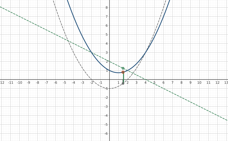
Interactive figure(f + g)(a) = f(a) + g(a): add the heights, one input at a timeDrag the Input a slider from -5 to 6.
XYZ Graph · viewer build 5edf91b
The two dashed curves are f(x) = x²/4 − 1 and g(x) = 2 − x/2; the solid curve is their sum f + g. At the input a set by the slider, the three marked heights are f(a), g(a) and (f + g)(a), and the two stacked vertical segments show the sum being assembled: the green segment is g(a) placed on top of the gray segment f(a), ending exactly at the solid curve. Slide a across the picture and the stacking is redone at every input, including places where one height is negative and the segments partly cancel, which is all function addition means.
Of course, in order to define by the formula , both and need to be defined in the first place; that is, must be in the domain of
and the domain of . You'll recall2 this means must be in the intersection of the domains of and . We define the following.
We put these definitions to work for us in the next example.
A few remarks are in order. First, in number parts through, we first encountered combinations of three functions despite Definition 5.1 only addressing combinations of two functions at a time. It turns out that function arithmetic inherits many of the same properties of real number arithmetic. For example, we showed above that . In general, given any three functions , , and , that is, function addition is assocative. To see this, choose an element common to the domains of , , and . Then
The key step to the argument is that which is true courtesy of the associative property of real number addition. And just like with real number addition, because function addition is associative, we may write instead of or even though, when it comes down to computations, we can only add two things together at a time.4
For completeness, we summarize the properties of function arithmetic in the theorem below. The proofs of the properties all follow along the same lines as the proof of the associative property and are left to the reader. We investigate some additional properties in the exercises.
In the next example, we decompose given functions into sums, differences, products and/or quotients of other functions. Note that there are infinitely many different ways to do this, including some trivial ones. For example, suppose we were instructed to decompose into a sum or difference of functions. We could write where and or we could choose and . More simply, we could write where and . We'll call this last decomposition a `trivial' decomposition. Likewise, if we ask for a decomposition of as a product, a nontrivial solution would be where and whereas a trivial solution would be and . In general, non-trivial solutions to decomposition problems avoid using the additive identity, , for sums and differences and the multiplicative identity, , for products and quotients.
The Arithmetic of Change
Recall the average rate of change of a function over the interval is the slope of the line connecting the two points and and is given by
For the purposes of this section, consider a function defined over an interval containing and where . The average rate of change of over the interval is thus given by the formula:5
Our aim in this section is to develop formulas which relate the rate of change of arithmetic combinations of functions to the rates of change of the component functions. Our first step is to study the difference operator `' and how it works with the standard arithmetic operations.
In general, if is some quantity which assumes two values in a particular order, say (the `first' or `initial' value) and (the `second' or `final' value), then . For example, if represents the temperature of an object before () heat is applied and after () heat is applied, represents the increase in temperature of the object.
In the context of functions and rates of change, is the function defined on the interval with and . Here, .
Suppose we have two quantities, and with and . What do we mean by ? The initial value of the sum would be the sum of the initial values . Likewise, the final value of the sum would be the sum of the final values . Hence:
A similar calculation gives .
Let's turn our attention to products. We have . We'd like to express in terms of and and there seems to be no way obvious way to do that. We take to some geometric reasoning for inspiration. Let's assume the all the quantities we're working with are positive.
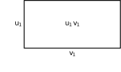
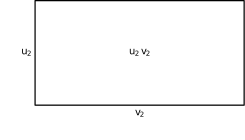
We imagine the product as being the area of a rectangle with width and length . Likewise, the product is the area of a (larger) rectangle with width and length .
Figure 5.20Figure 5.21
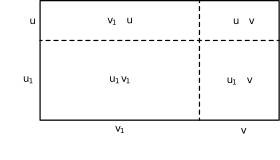
From , we get and, likewise, . Doing so allows us to decompose the larger rectangle into four smaller rectangles.
Figure 5.22
Using this schematic, we see the area is the sum of the areas of four smaller rectangles:
Hence, .
To prove this formula holds in general, we can substitute and into and simplify. We leave the details to the reader.6
Next, we turn our attention to quotients. We begin with: .
Instead of appealing to geometric reasoning here,7 we take a cue from the previous discussion and substitute and and set about getting a common denominator:
We summarize these results in the following theorem.
You'll note we've called out a special case for the Product Rule, the Constant Multiple Rule. If one of the factors is a constant, , then (since constants don't change.)
In the following example, we use the Quotient Rule for Change to help approximate the propagated error when using measured quantities (with associated uncertainties) in calculations.8
In order to establish formulas for the average rate of change for functions, we substitute for and for and divide each of the expressions in Theorem 5.2 by . For example, if we to find an expression for the average rate of change of in terms of , , and their respective average rates of change:
Note that with the last term, we may associate the `' with either of the factors in the numerator:
Either way, we've managed to express the average rate of change of the function in terms of the changes and rates of change of and .
In the result below, we abbreviate the average rate of change as `ARoC' for convenience.
Our final example revisits the scenario in Exercise in Section 2.1.
Note that in Example 5.2.4, since , the average rate of change for the cost moving from producing to systems, is the same numerical value as the additional cost incurred by producing the st system, . The same goes for the revenue and profit calculations. This is the concept of marginal analysis is studied at length in Economics and Business Calculus classes.10 For us, it's time for some Exercises.
Exercises
In Exercises -, use the pair of functions and to find the following values if they exist.
and
and
and
and
and
and
and
and
and
and
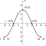
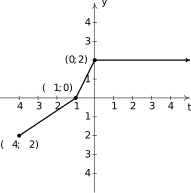
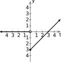
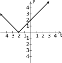
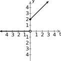
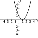
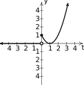
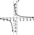
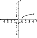
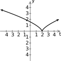
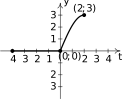
Exercises - refer to the functions and whose graphs are below.
Figure 5.24Figure 5.25
Find the domains of , , , and .
In Exercises -, let be the function defined by
and let be the function defined by
Compute the indicated value if it exists.
In Exercises -, use the pair of functions and to find the domain of the indicated function then find and simplify an expression for it.
and
and
and
and
and
and
and
and
and
and
In Exercises -, write the given function as a nontrivial decomposition of functions as directed.
For , find functions and so that .
For , find functions and so that .
For , find functions and so that .
For , find functions and so .
For , find functions and so .
Can be decomposed as where and ?
Discuss with your classmates how to phrase the quantities revenue and profit in Definition 1.12 terms of function arithmetic as defined in Definition 5.1.
In this exercise, we explore decomposing a function into its positive and negative parts. Given a function , we define the positive part of , denoted and negative part of , denoted by:
Using a graphing utility, graph each of the functions below along with and .
Why is called the `positive part' of and called the `negative part' of ?
Show that .
Use Definition 1.9 to rewrite the expressions for and as piecewise defined functions.
Let be the unit step function defined in Exercise in Section 1.2. For each function below:
Write as a piecewise-defined function.
Graph and .
Write a general formula for for a function . (Assume the domain of is .)
Explain how to obtain the graph of from .
The function is used to model a change in state from `off' to `on' (like flipping a light switch.) How does this relate to your observations?
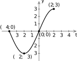
Use the graph of below to graph .
Figure 5.26
Use Example 5.2.3 as a guide to help find the following uncertainties.
A chemist combines the solutions from two graduated cylinders into a beaker. The volume of the first solution, , an acid, is read as milliliters (mL). The volume of the second solution, a base, , is measured to be mL. Estimate the percent propagated error in calculating the volume of the combined solution as mL.
A student measures the length, , and width, , of a piece of paper. They find millimeters (mm) mm. Estimate the percent propagated error in calculating the area of the piece of paper as .
An airplane passenger observers a car travel a distance feet (ft) in time seconds (s). Estimate the percent propagated error in calculating the speed of the car as .
Let us return to Example 5.2.4 where denotes the cost, in dollars, of producing PortaBoy game systems. Recall the average cost11 is defined as , , is the cost per item.
Find and interpret .
Define the marginal cost
. Find and interpret .
How do your answers to parts and compare?
Graph with help from a graphing utility. What is happening graphically near ?
Use Theorem 5.3 to show that, in general, when .
HINT: Note that, by definition, when .
Hence, in this case …
Answers
For and
For and
For and
For and
For and
For and
For and
For and
For and
is undefined.
For and
The domains of , and are all . The domain of is and the domain of is .
does not exist
does not exist
For and
Domain:
Domain:
Domain:
Domain:
For and
Domain:
Domain:
Domain:
Domain:
For and
Domain:
Domain:
Domain:
Domain:
For and
Domain:
Domain:
Domain:
Domain:
For and
Domain:
Domain:
Domain:
Domain:
For and
Domain:
Domain:
Domain:
Domain:
For and
Domain:
Domain:
Domain:
Domain:
For and
Domain:
Domain:
Domain:
Domain:
For and
Domain:
Domain:
Domain:
Domain:
For and
Domain:
Domain:
Domain:
Domain:
One solution is and .
One solution is and .
One solution is and
One solution is and .
One solution is and .
No. The equivalence does not hold when .
.
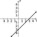
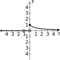
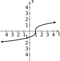
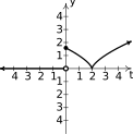
Figure 5.27Figure 5.28
Figure 5.29Figure 5.30
Figure 5.31Figure 5.32
Figure 5.33Figure 5.34 - note the hole at
Figure 5.35Figure 5.36
Figure 5.37Figure 5.38
The graph of is for and for .
The unit step function keeps the function `off' until then turns the function `on' for .
Figure 5.39
.
.
.
.
. When making systems, the cost per system is approximately .
. It costs an additional to make the th system.
and appear to be `pretty close.'
The graph has a local (absolute) minimum right near .
Per Theorem 5.3, since
If , then the numerator, . Solving for , we get . If we are working with a whole number of items, the smallest meaningful value of is , in which case . Hence, when , that is, when the marginal cost and average cost are the same. At this point, the graph of levels off (at a minumum.)12 Can you reason why this creates a minimum?
Adapted from Precalculus with Integrated Calculus, edition 4i, by Carl Stitz and Jeff Zeager (stitz-zeager.com), licensed under CC BY-NC-SA 3.0. Changes were made: reformatted as an accessible XYZ web edition. License: CC-BY-NC-SA-3.0.
These eBooks are a prerelease and are not yet certified conformant with WCAG 2.1 AA or any other accessibility standard. Every page is built against an automated accessibility gate, and our target for the published editions is WCAG 2.2 Level AA. If something is unusable, please tell us.