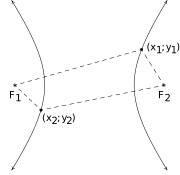
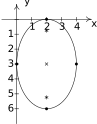
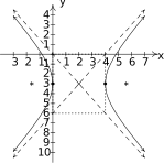
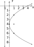
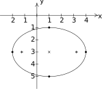
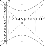
In the definition of an ellipse, Definition 7.4, we fixed two points called foci and looked at points whose distances to the foci always added to a constant distance . Those prone to syntactical tinkering may wonder what, if any, curve we'd generate if we replaced added with subtracted. The answer is a hyperbola.
Figure 7.65
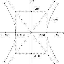
In the figure above:
and
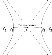
Note that the hyperbola has two parts, called branches. The center of the hyperbola is the midpoint of the line segment connecting the two foci. The transverse axis of the hyperbola is the line segment connecting two opposite ends of the hyperbola which also contains the center and foci. The vertices of a hyperbola are the points of the hyperbola which lie on the transverse axis. In addition, we will show momentarily that there are lines called asymptotes which the branches of the hyperbola approach for large and values. They serve as guides to the graph. In pictures,
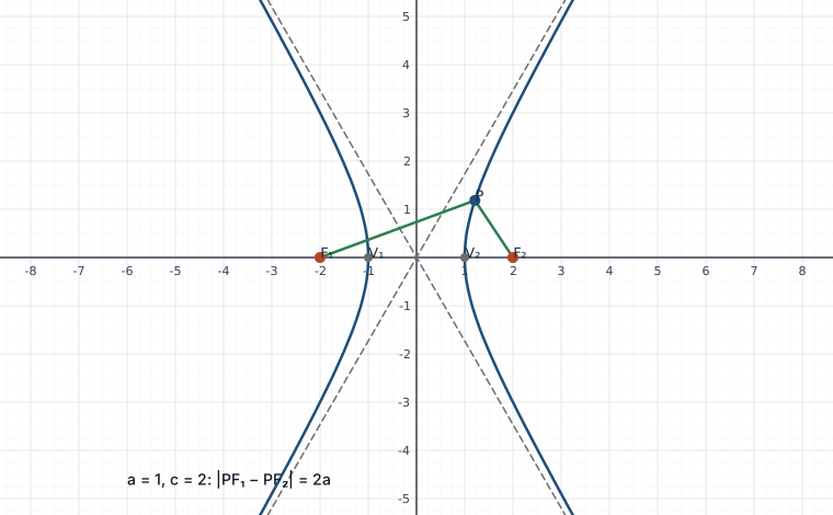
Interactive figureFoci, vertices and asymptotes of x²/a² − y²/b² = 1Move the Vertex distance a, Focal distance c and Position of P on the right branch sliders.
A hyperbola centred at the origin with vertices (±a, 0) and foci (±c, 0), both on sliders (c stays larger than a). The dashed lines are the asymptotes y = ±(b/a)x with b² = c² − a², which the branches approach but never meet; the point P rides the right branch, and the two segments to the foci differ in length by exactly 2a wherever P is — the difference that defines the curve, as the sum defines the ellipse. Move c toward a and the branches close toward the x-axis; move it away and they open toward the asymptotes' steeper slopes.Figure 7.66
A hyperbola with center ; foci , ; and vertices , and asymptotes (dashed)
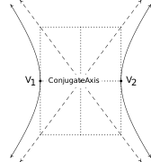
Before we derive the standard equation of the hyperbola, we need to discuss one further parameter, the conjugate axis of the hyperbola. The conjugate axis of a hyperbola is the line segment through the center which is perpendicular to the transverse axis and has the same length as the line segment through a vertex which connects the asymptotes. In pictures we have
Figure 7.67
Note that in the diagram, we can construct a rectangle using line segments with lengths equal to the lengths of the transverse and conjugate axes whose center is the center of the hyperbola and whose diagonals are contained in the asymptotes. This guide rectangle, much akin to the one we saw Section 7.4 to help us graph ellipses, will aid us in graphing hyperbolas.
Suppose we wish to derive the equation of a hyperbola. For simplicity, we shall assume that the center is , the vertices are and and the foci are and . We label the endpoints of the conjugate axis and . (Although does not enter into our derivation, we will have to justify this choice as you shall see later.) As before, we assume , , and are all positive numbers. Schematically we have
Figure 7.68
Since is on the hyperbola, it must satisfy the conditions of Definition 7.6. That is, the distance from to minus the distance from to must equal the fixed distance . Since all these points lie on the -axis, we get
In other words, the fixed distance from the definition of the hyperbola is actually the length of the transverse axis! (Where have we seen that type of coincidence before?) Now consider a point on the hyperbola. Applying Definition 7.6, we get
Using the same arsenal of Intermediate Algebra weaponry we used in deriving the standard formula of an ellipse, Equation 7.4, we arrive at the following.1
What remains is to determine the relationship between , and . To that end, we note that since and are both positive numbers with , we get so that is a negative number. Hence, is a positive number. For reasons which will become clear soon, we re-write the equation by solving for to get
As and attain very large values, the quantity so that . By setting we get . This shows that as grows large. Thus are the asymptotes to the graph as predicted and our choice of labels for the endpoints of the conjugate axis is justified. In our equation of the hyperbola we can substitute which yields
The equation above is for a hyperbola whose center is the origin and which opens to the left and right. If the hyperbola were centered at a point , we would get the following.
If the roles of and were interchanged, then the hyperbola's branches would open upwards and downwards and we would get a `vertical' hyperbola.
The values of and determine how far in the and directions, respectively, one counts from the center to determine the rectangle through which the asymptotes pass. In both cases, the distance from the center to the foci, , as seen in the derivation, can be found by the formula . Lastly, note that we can quickly distinguish the equation of a hyperbola from that of a circle or ellipse because the hyperbola formula involves a difference of squares where the circle and ellipse formulas both involve the sum of squares.
As with the other conic sections, an equation whose graph is a hyperbola may not be given in either of the standard forms. To rectify that, we have the following.
To Write the Equation of a Hyperbola in Standard Form
Group the same variables together on one side of the equation and position the constant on the other side
Complete the square in both variables as needed
Divide both sides by the constant term so that the constant on the other side of the equation becomes
Hyperbolas can be used in so-called `trilateration,' or `positioning' problems. The procedure outlined in the next example is the basis of the (now virtually defunct) LOng Range Aid to Navigation (LORAN for short) system.3
In our previous example, we did not have enough information to pin down the exact location of Sasquatch. To accomplish this, we would need a third observer.
Each of the conic sections we have studied in this chapter result from graphing equations of the form for different choices of , , , , and6
. While we've seen examples7 demonstrate how to convert an equation from this general form to one of the standard forms, we close this chapter with some advice about which standard form to choose.8
Strategies for Identifying Conic Sections
Suppose the graph of equation is a non-degenerate conic section.9
If just one variable is squared, the graph is a parabola. Put the equation in the form of Equation 7.2 (if is squared) or Equation 7.3 (if is squared).
If both variables are squared, look at the coefficients of and , and .
If , the graph is a circle. Put the equation in the form of Equation 7.1.
If but and have the same sign, the graph is an ellipse. Put the equation in the form of Equation 7.4.
If and have the different signs, the graph is a hyperbola. Put the equation in the form of either Equation 7.6 or Equation 7.7.
Exercises
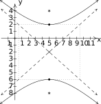
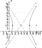
In Exercises -, graph the hyperbola. Find the center, the lines which contain the transverse and conjugate axes, the vertices, the foci and the equations of the asymptotes.
In Exercises -, put the equation in standard form. Find the center, the lines which contain the transverse and conjugate axes, the vertices, the foci and the equations of the asymptotes.
In Exercises -, find the standard form of the equation of the hyperbola which has the given properties.
Center , Vertex , Focus
Vertex , Vertex , Focus
Foci , Vertices .
Foci , length of the Conjugate Axis
Vertices , ; Endpoints of the Conjugate Axis ,
Vertex , Asymptotes
In Exercises -, find the standard form of the equation using the guidelines on page Section 7.5 and then graph the conic section.
The graph of a vertical or horizontal hyperbola clearly fails the Vertical Line Test, Theorem 1.1, so the equation of a vertical of horizontal hyperbola does not define as a function of .10 However, much like with circles, horizontal parabolas and ellipses, we can split a hyperbola into pieces, each of which would indeed represent as a function of . With the help of your classmates, use your calculator to graph the hyperbolas given in Exercises - above. How many pieces do you need for a vertical hyperbola? How many for a horizontal hyperbola?
The location of an earthquake's epicenter the point on the surface of the Earth directly above where the earthquake actually occurred can be determined by a process similar to how we located Sasquatch in Example 7.5.5. (As we said back in Exercise in Section 6.1, earthquakes are complicated events and it is not our intent to provide a complete discussion of the science involved in them. Instead, we refer the interested reader to a course in Geology or the U.S. Geological Survey's Earthquake Hazards Program found here.) Our technique works only for relatively small distances because we need to assume that the Earth is flat in order to use hyperbolas in the plane.11 The P-waves (“P” stands for Primary) of an earthquake in Sasquatchia travel at 6 kilometers per second.12 Station A records the waves first. Then Station B, which is 100 kilometers due north of Station A, records the waves 2 seconds later. Station C, which is 150 kilometers due west of Station A records the waves 3 seconds after that (a total of 5 seconds after Station A). Where is the epicenter?
The notion of eccentricity introduced for ellipses in Definition 7.5 in Section 7.4 is the same for hyperbolas in that we can define the eccentricity of a hyperbola as
With the help of your classmates, explain why for any hyperbola.
Find the equation of the hyperbola with vertices and eccentricity .
With the help of your classmates, find the eccentricity of each of the hyperbolas in Exercises -. What role does eccentricity play in the shape of the graphs?
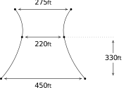
On page in Section 7.3, we discussed paraboloids of revolution when studying the design of satellite dishes and parabolic mirrors. In much the same way, `natural draft' cooling towers are often shaped as hyperboloids of revolution. Each vertical cross section of these towers is a hyperbola. Suppose the a natural draft cooling tower has the cross section below. Suppose the tower is 450 feet wide at the base, 275 feet wide at the top, and 220 feet at its narrowest point (which occurs 330 feet above the ground.) Determine the height of the tower to the nearest foot.
Figure 7.76
With the help of your classmates, research the Cassegrain Telescope. It uses the reflective property of the hyperbola as well as that of the parabola to make an ingenious telescope.
With the help of your classmates show that if determines a non-degenerate conic13 then
means that the graph is a hyperbola
means that the graph is a parabola
means that the graph is an ellipse or circle
NOTE: This result will be generalized in Theorem 11.11 in Section 11.6.1.
Answers
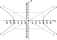
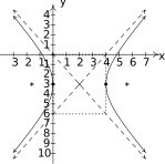
Center Transverse axis on Conjugate axis on Vertices Foci Asymptotes
Figure 7.77
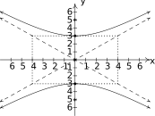
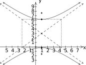
Center Transverse axis on Conjugate axis on Vertices Foci Asymptotes
Figure 7.78
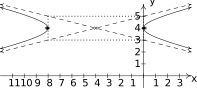
Center Transverse axis on Conjugate axis on Vertices Foci Asymptotes
Figure 7.79
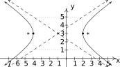
Center Transverse axis on Conjugate axis on Vertices Foci Asymptotes
Figure 7.80
Center Transverse axis on Conjugate axis on Vertices Foci Asymptotes
Figure 7.81
Center Transverse axis on Conjugate axis on Vertices Foci Asymptotes
Figure 7.82
Center Transverse axis on Conjugate axis on Vertices Foci Asymptotes
Figure 7.83
Center Transverse axis on Conjugate axis on Vertices Foci Asymptotes
Figure 7.84
Center Transverse axis on Conjugate axis on Vertices Foci Asymptotes
Center Transverse axis on Conjugate axis on Vertices Foci Asymptotes
Center Transverse axis on Conjugate axis on Vertices Foci Asymptotes
Center Transverse axis on Conjugate axis on Vertices Foci Asymptotes
Figure 7.85
Figure 7.86
Figure 7.87
Figure 7.88
Figure 7.89
The graph is the point only.
Figure 7.90
There is no graph.
There is no graph.
Figure 7.91
By placing Station A at and Station B at , the two second time difference yields the hyperbola with foci A and B and center . Placing Station C at and using foci A and C gives us a center of and the hyperbola . The point of intersection of these two hyperbolas which is closer to A than B and closer to A than C is so that is the epicenter.
.
The tower may be modeled (approximately)14 by . To find the height, we plug in which yields or . Since the top of the tower is above the narrowest point, we get the tower is approximately 469 feet tall.
Adapted from Precalculus, 3rd corrected edition, by Carl Stitz and Jeff Zeager (stitz-zeager.com), licensed under CC BY-NC-SA 3.0. Changes were made: reformatted as an accessible XYZ web edition. License: CC-BY-NC-SA-3.0.
These eBooks are a prerelease and are not yet certified conformant with WCAG 2.1 AA or ADA Title II. Every page is built against an automated accessibility gate, and the published editions will meet ADA Title II requirements when they release in late September 2026. If something is unusable, please tell us.