
7.6 Normal Approximation to the Binomial
In the section on the history of the normal distribution, we saw that the normal distribution can be used to approximate the binomial distribution. This section shows how to compute these approximations.
Let's begin with an example. Assume you have a fair coin and wish to know the probability that you would get 8 heads out of 10 flips. The binomial distribution has a mean of μ = Nπ = (10)(0.5) = 5 and a variance of σ2 = Nπ(1-π) = (10)(0.5)(0.5) = 2.5. The standard deviation is therefore 1.5811. A total of 8 heads is (8 - 5)/1.5811 = 1.897 standard deviations above the mean of the distribution. The question then is, "What is the probability of getting a value exactly 1.897 standard deviations above the mean?" You may be surprised to learn that the answer is 0: The probability of any one specific point is 0. The problem is that the binomial distribution is a discrete probability distribution, whereas the normal distribution is a continuous distribution.
The solution is to round off and consider any value from 7.5 to 8.5 to represent an outcome of 8 heads. Using this approach, we figure out the area under a normal curve from 7.5 to 8.5. The area in green in Figure 1 is an approximation of the probability of obtaining 8 heads.
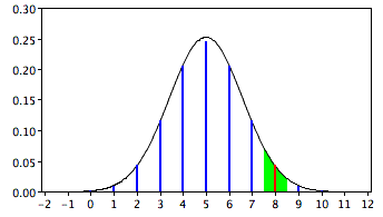
The solution is therefore to compute this area. First we compute the area below 8.5 and then subtract the area below 7.5.
The results of using the normal area calculator to find the area below 8.5 are shown in Figure 2. The results for 7.5 are shown in Figure 3.
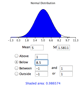
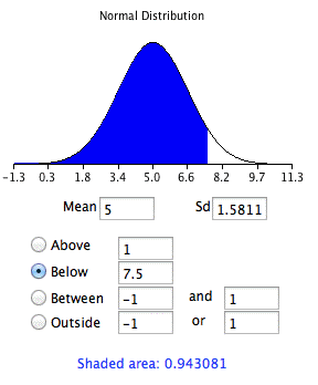
The difference between the areas is 0.044, which is the approximation of the binomial probability. For these parameters, the approximation is very accurate. The demonstration in the next section allows you to explore its accuracy with different parameters.
If you did not have the normal area calculator, you could find the solution using a table of the standard normal distribution (a Z table) as follows:
- Find a Z score for 8.5 using the formula Z = (8.5 - 5)/1.5811 = 2.21.
- Find the area below a Z of 2.21 = 0.987.
- Find a Z score for 7.5 using the formula Z = (7.5 - 5)/1.5811 = 1.58.
- Find the area below a Z of 1.58 = 0.943.
- Subtract the value in step 4 from the value in step 2 to get 0.044.
The same logic applies when calculating the probability of a range of outcomes. For example, to calculate the probability of 8 to 10 flips, calculate the area from 7.5 to 10.5.
The accuracy of the approximation depends on the values of N and π. A rule of thumb is that the approximation is good if both Nπ and N(1-π) are both greater than 10.
Adapted from Online Statistics Education: A Multimedia Course of Study (onlinestatbook.com), Project Leader: David M. Lane, Rice University. Developed with NSF support. The original work is in the public domain; it is cited here at the authors' request. Changes were made: reformatted as an accessible XYZ web edition with native MathML. License: Public-Domain.