Areas under portions of a normal distribution
can be computed by using calculus. Since this is a non-mathematical
treatment of statistics, we will rely on computer programs and
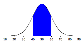
tables to determine these areas. Figure 1 shows a normal distribution
with a mean of 50 and a standard deviation of 10. The shaded area
between 40 and 60 contains 68% of the distribution.
Figure 1. Normal distribution with a mean
of 50 and standard deviation of 10. 68% of the area is within
one standard deviation (10) of the mean (50).
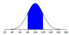
Figure 2 shows a normal distribution with a mean
of 100 and a standard deviation of 20. As in Figure 1, 68% of
the distribution is within one standard deviation of the mean.
Figure 2. Normal distribution with a mean
of 100 and standard deviation of 20. 68% of the area is
within one standard deviation (20) of the mean (100).
The normal distributions shown in Figures 1 and
2 are specific examples of the general rule that 68% of the area
of any normal distribution is within one standard deviation of
the mean.
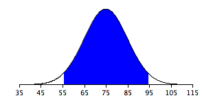
Figure 3 shows a normal distribution with a mean
of 75 and a standard deviation of 10. The shaded area contains
95% of the area and extends from 55.4 to 94.6. For all normal
distributions, 95% of the area is within 1.96 standard deviations
of the mean. For quick approximations, it is sometimes useful
to round off and use 2 rather than 1.96 as the number of standard
deviations you need to extend from the mean so as to include 95%
of the area.
Figure 3. A normal distribution with a
mean of 75 and a standard deviation of 10. 95% of the area
is within 1.96 standard deviations of the mean.
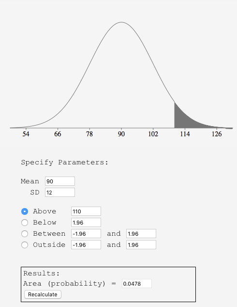
The normal calculator can be used to calculate areas under
the normal distribution. For example, you can use it to find the proportion of a normal
distribution with a mean of 90 and a standard deviation of 12
that is above 110. Set the mean to 90 and the standard deviation
to 12. Then enter "110" in the box to the right of the
radio button "Above." At the bottom of the display you
will see that the shaded area is 0.0478. See if you can use the
calculator to find that the area between 115 and 120 is 0.0124.
Figure 4. Display from calculator showing
the area above 110.
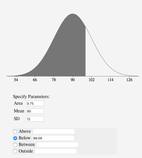
Say
you wanted to find the score corresponding to the 75th percentile
of a normal distribution with a mean of 90 and a standard deviation
of 12. Using the inverse normal calculator, you enter the parameters as shown in Figure 5 and find that the area below 98.09 is 0.75.
Figure 5. Display from normal calculator showing
that the 75th percentile is 98.09.
Normal and Inverse Normal Calculator
Adapted from Online Statistics Education: A Multimedia Course of Study (onlinestatbook.com), Project Leader: David M. Lane, Rice University. Developed with NSF support. The original work is in the public domain; it is cited here at the authors' request. Changes were made: reformatted as an accessible XYZ web edition with native MathML. License: Public-Domain.
These eBooks are a prerelease and are not yet certified conformant with WCAG 2.1 AA or ADA Title II. Every page is built against an automated accessibility gate, and the published editions will meet ADA Title II requirements when they release in late September 2026. If something is unusable, please tell us.