
3.8 Mean and Median Demo
This section is an interactive demonstration. The live simulation runs on the original site: open the demonstration at onlinestatbook.com.
Learning Objectives
- Understand how the mean and median change with different distributions.
Instructions
This demonstration shows how the relative size of the mean and the median depends on the skew of the distribution.
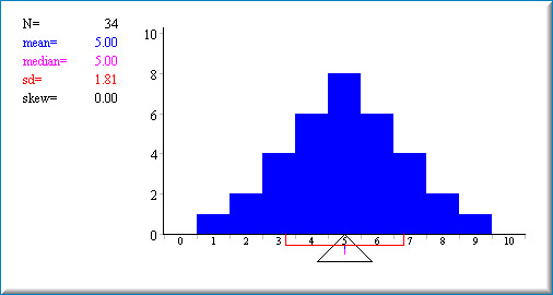
The demonstration begins by showing a histogram of a symmetric distribution (no skew). The mean and median are both 5.0. The mean is shown on the histogram as a small blue line; the median is shown as a small purple line. The standard deviation is 1.81. A red line extends one sd in each direction from the mean. The standard deviation is calculated assuming the data portrayed in the graph represent the entire population.
You can change the values of the data set by "painting" the histogram with the mouse.
Change the distribution in various ways and note how the skew affects whether the mean is bigger than the median or vice versa.
Illustrated Instructions
The simulation starts out with a symmetrical distribution. As can be seen seen in the screenshot below the mean and median are equal and there is 0 skew.
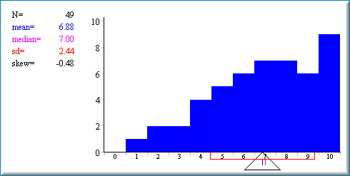
The distribution can be changed "painting" it with the mouse. Below is an example of a negatively skewed distribution.
Note that the mean and median are no longer equal to each other. Trying painting several different types of distributions to see how mean and median values are affected relative to each other.
"Paint" the distributon with the mouse and observe the effects. The mean and median are shown to the left and also as small vertical bars below the X-axis. The mean is in blue and the median is in pink.
Adapted from Online Statistics Education: A Multimedia Course of Study (onlinestatbook.com), Project Leader: David M. Lane, Rice University. Developed with NSF support. The original work is in the public domain; it is cited here at the authors' request. Changes were made: reformatted as an accessible XYZ web edition with native MathML. License: Public-Domain.