3.10 Comparing Measures

How do the various measures of central tendency compare with each other? For symmetric distributions, the mean, median, trimean, and trimmed mean are equal, as is the mode except in bimodal distributions. Differences among the measures occur with skewed distributions. Figure 1 shows the distribution of 642 scores on an introductory psychology test. Notice this distribution has a slight positive skew.

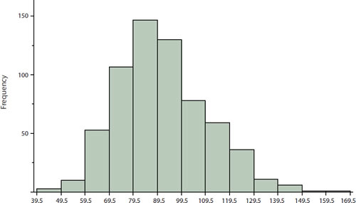
Histogram of 642 psychology test scores grouped in intervals of 10 with class boundaries labeled 39.5 through 169.5. Frequencies rise from near 0 at 39.5-49.5 to a peak of about 147 in the 79.5-89.5 interval, then fall through about 130, 78, 59, 36 down to single digits above 139.5. The distribution is unimodal and skewed slightly to the right. — Figure 1. A distribution with a positive skew.

Measures of central tendency are shown in Table 1. Notice they do not differ greatly, with the exception that the mode is considerably lower than the other measures. When distributions have a positive skew, the mean is typically higher than the median, although it may not be in bimodal distributions. For these data, the mean of 91.58 is higher than the median of 90. Typically the trimean and trimmed mean will fall between the median and the mean, although in this case, the trimmed mean is slightly lower than the median. The geometric mean is lower than all measures except the mode.

Table 1. Measures of central tendency

for the test scores.

Measure	Value
Mode Median Geometric Mean Trimean Mean trimmed 50% Mean	84.00 90.00 89.70 90.25 89.81 91.58

The distribution of baseball salaries (in 1994) shown in Figure 2 has a much more pronounced skew than the distribution in Figure 1.

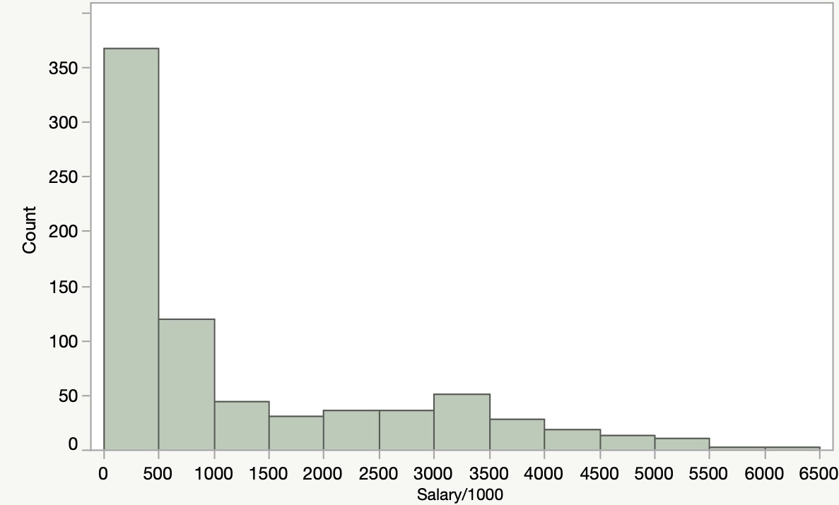
Histogram of major league baseball salaries, x-axis Salary/1000 from 0 to 6500 in steps of 500 and y-axis Count: about 367 players in the lowest bin, about 120 in the next, then about 45, 30, 36, 36, a secondary rise to about 51 near 3000-3500, and a thin tail of about 28, 18, 13, 9 down to nearly 0 above 5500 — a very large positive skew. — Figure 2. A distribution with a very large positive skew. This histogram shows the salaries of major league baseball players (in thousands of dollars: 250 equals 250,000).

Table 2 shows the measures of central tendency for these data. The large skew results in very different values for these measures. No single measure of central tendency is sufficient for data such as these. If you were asked the very general question: "So, what do baseball players make?" and answered with the mean of $1,183,000, you would not have told the whole story since only about one third of baseball players make that much. If you answered with the mode of $250,000 or the median of $500,000, you would not be giving any indication that some players make many millions of dollars. Fortunately, there is no need to summarize a distribution with a single number. When the various measures differ, our opinion is that you should report the mean, median, and either the trimean or the mean trimmed 50%. Sometimes it is worth reporting the mode as well. In the media, the median is usually reported to summarize the center of skewed distributions. You will hear about median salaries and median prices of houses sold, etc. This is better than reporting only the mean, but it would be informative to hear more statistics.

Table 2. Measures of central tendency for baseball salaries (in thousands of dollars).

Measure	Value
Mode Median Geometric Mean Trimean Mean trimmed 50% Mean	250 500 555 792 619 1,183

Adapted from Online Statistics Education: A Multimedia Course of Study (onlinestatbook.com), Project Leader: David M. Lane, Rice University. Developed with NSF support. The original work is in the public domain; it is cited here at the authors' request. Changes were made: reformatted as an accessible XYZ web edition with native MathML. License: Public-Domain.