10.3 Test for Independence

Use the chi-square test for independence to test the independence of two categorical variables. Remember, qualitative data is collected on individuals that are categories or names. Then you would count how many of the individuals had particular qualities. An example is that there is a theory that there is a relationship between breastfeeding and having autism spectrum disorder (ASD). To determine if there is a relationship, researchers could collect the time-period that a mother breastfed her child and if that child was diagnosed with ASD. Then you would have a table containing this information. Now you want to know if each cell is independent of each other cell. Remember, independence says that one event does not affect another event. Here it means that having ASD is independent of being breastfed. What you really want is to see if they are dependent (not independent). In other words, does one affect the other? If you were to do a hypothesis test, this is your alternative hypothesis and the null hypothesis is that they are independent. There is a hypothesis test for this and it is called the chi-square test for independence.

Finding the test statistic involves several steps. First, the data is collected, counted, and then organized into a contingency table. These values are known as the observed frequencies, and the symbol for an observed frequency is $O$ . Total each row and column.

The null hypothesis is that the two variables are independent. If two events are independent then $P (B) = P (B | A)$ and we can use the multiplication rule for independent events, to calculate the probability that variable $A$ and $B$ as the $P (A and B) = P (A) \cdot P (B)$ . Remember in a hypothesis test, you assume that $H sub 0$ is true, the two variables are assumed to be independent.

$\begin{matrix} P (A and B) = P (A) \cdot P (B) if A and B are independent \\ = \frac{Number of ways A can happen}{Total number of individuals} \cdot \frac{Number of ways B can happen}{Total number of individuals} \\ = \frac{Row Total}{n} \cdot \frac{Column Total}{n} \end{matrix}$

General two-way table layout with Variable 1 columns B and Not B and Variable 2 rows A and Not A; the cells hold P(A and B), P(A and Not B), P(Not A and B), and P(Not A and Not B), with row totals for A and Not A, column totals for B and Not B, and grand total n.

Now you want to find out how many individuals you expect to be in a certain cell. To find the expected frequencies, you just need to multiply the probability of that cell times the total number of individuals. Do not round the expected frequencies.

$\begin{matrix} Expected frequency (cell A and B) = E (A and B) \\ = n (\frac{Row Total}{n} \cdot \frac{Column Total}{n}) = \frac{Row Total \cdot Column Total}{n} \end{matrix}$

If the variables are independent, the expected frequencies and the observed frequencies should be the same.

The test statistic here will involve looking at the difference between the expected frequency and the observed frequency for each cell. Then you want to find the “total difference” of all of these differences. The larger the total, the smaller the chances that you could find that test statistic given that the assumption of independence is true. That means that the assumption of independence is not true.

How do you find the test statistic? First, compute the differences between the observed and expected frequencies. Because some of these differences will be positive and some will be negative, you need to square these differences. These squares could be large just because the frequencies are large, so you need to divide by the expected frequencies to scale them. Then finally add up all of these fractional values. This process finds the variance, and we use a chi-square distribution to find the critical value or p-value. Hence, sometimes this test is called a chi-square test.

Example 1

Is there a relationship between autism spectrum disorder (ASD) and breastfeeding? To determine if there is, a researcher asked mothers of ASD and non-ASD children to say what time-period they breastfed their children. Does the data provide enough evidence to show that breastfeeding and ASD are independent? Test at the 1% level.

(Schultz, Klonoff-Cohen, Wingard, Askhoomoff, Macera, Ji & Bacher, 2006.)

Show solution

The question is asking if breastfeeding and ASD are independent. The correct hypothesis is:

$H sub 0:$ Autism spectrum disorder and length of breastfeeding are independent.

$H sub 1:$ Autism spectrum disorder and length of breastfeeding are dependent.

There are 2 rows and 4 columns of data. We must compute the Expected count for each of the $2 \times 4 = 8$ cells.

It will be helpful to make a table for the expected counts and another one for each of the $\frac{(O - E)^{2}}{E}$ values to aid in computing the test statistic.

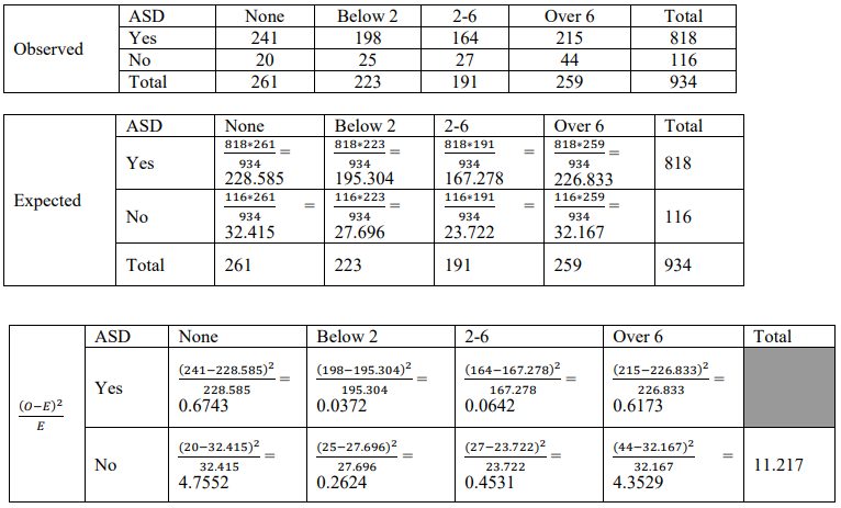
Three stacked tables for the ASD and breastfeeding test: the observed counts; the expected counts computed as row total times column total over 934, giving 228.585, 195.304, 167.278, 226.833 for Yes and 32.415, 27.696, 23.722, 32.167 for No; and the (O−E)²/E values 0.6743, 0.0372, 0.0642, 0.6173 and 4.7552, 0.2624, 0.4531, 4.3529, which sum to the test statistic 11.217.

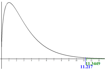
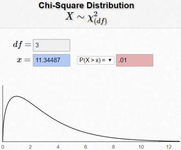
The test statistic is the sum of all eight $\frac{(O - E)^{2}}{E}$ values: $χ^{2} = \sum \frac{(O - E)^{2}}{E} = 11.217$ .

The critical value for a right-tailed $χ^{2}$ -test with degrees of freedom $df = (R - 1) (C - 1) = (2 - 1) (4 - 1) = 3$ is found using a $χ^{2}$ -distribution $α equals 0.01$ right-tail area. The critical value is $χ^{2}$ = CHISQ.INV.RT(0.01,3) = 11.3449. See Figure 10-5.

Right-skewed chi-square curve with the critical value 11.3449 marked in green on the axis and the test statistic 11.217 marked in blue just to its left, outside the small shaded rejection region in the right tail. — Figure 10-5: Values of $χ^{2}$ and $χ_{α}^{2}$ on a $χ^{2}$ -test with $df equals 3$ and $α equals 0.01$ .

Alternatively, use the online calculator: https://homepage.divms.uiowa.edu/~mbognar/applets/chisq.html.

Online chi-square distribution calculator titled Chi-Square Distribution with inputs df = 3, x = 11.34487, and P(X > x) = .01, above a plotted right-skewed chi-square curve on an axis from 0 to 12.

Since the test statistic $χ squared equals 11.217$ is not in the rejection area, our decision is to fail to reject $H sub 0$ .

There is not enough evidence to show a relationship between autism spectrum disorder and breastfeeding.

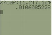
TI-84 calculator screen showing a χ²cdf command with lower bound 11.217 returning .0106085228.

If we were asked to find the p-value, you would just find the area to right of the test statistic (always a right-tailed test) using your calculator or Excel. This gives a p-value = 0.0106, which is more than $α equals 0.01$ ; therefore, we do not reject H₀.

You can also use the $χ^{2}$ -Test shortcut keys on your calculator to get a p-value, see directions below.

TI-84: Press the [2^nd] then [MATRX] key. Arrow over to the EDIT menu and 1:[A] should be highlighted, press the [ENTER] key. For a $m \times n$ contingency table, type in the number of rows $(m)$ and the number of columns $(n)$ at the top of the screen so that it looks like this: MATRIX[A] $m \times n$ . For a $2 times 4$ contingency table, the top of the screen would look like this: MATRIX[A] $2 times 4$ . As you hit [ENTER], the table will automatically widen to the size you put in. Now enter all of the observed values in their proper positions. Then press the [STAT] key, arrow over to the [TESTS] menu, arrow down to the option [C: $χ^{2}$ -Test] and press the [ENTER] key. Leave the default as Observed:[A] and Expected:[B], arrow down to [Calculate] and press the [ENTER] key.

The calculator returns the $χ^{2}$ -test statistic and the p-value.

If you go back to the matrix menu [2^nd] then [MATRX] key, arrow over to EDIT and choose 2:[B], you will see all of the expected values.

Five TI-84 screens for the matrix χ²-Test: the matrix EDIT menu, matrix [A] entered as a 2 by 4 table of observed counts ending with cell 2,4 = 44, the TESTS menu with C:χ²-Test selected, the inputs Observed:[A] and Expected:[B], and the output χ²=11.21668801, p=.0106100514, df=3.

TI-89: First you need to create the matrix for the observed values: Press [Home] to return to the Home screen, press [Apps] and select Data/Matrix Editor. A menu is displayed, select 3:New. The New dialog box is displayed. Press the right arrow key to highlight 2:Matrix, and press [ENTER] to choose Matrix type. Press the down arrow key to highlight 1:Main, and press [ENTER], to choose main folder. Press the down arrow key, and then enter the letter $o$ for the name in the Variable field. Enter 2 for Row dimension and 4 for Column dimension. Press [ENTER] to display the matrix editor. Enter the observed value (do not include total row or column). Important: Next time you use this test instead of option 3:New, choose 2: Open. The open dialog box is displayed. Press the right arrow key to highlight 2:Matrix, and press [ENTER] to choose Matrix type. Press the down arrow key to make sure you are in the Main folder and that your variable says $o$ . Press [Apps], and then select Stats/List Editor. To display the Chi-square 2-Way dialog box, press 2^nd then F6 [Tests], then select 8: Chi-2 2-way. Enter in in the Observed Mat: o; leave the other rows alone: Store Expected to: statvars\e; Store CompMat to: statvars\c. This will store the expected values in the matrix folder statvars with the name expmat, and the $open parenthesis o minus e close parenthesis squared / e$ values in the matrix compmat. Press the [ENTER] key to calculate. The calculator returns the $χ^{2}$ -test statistic and the p-value. 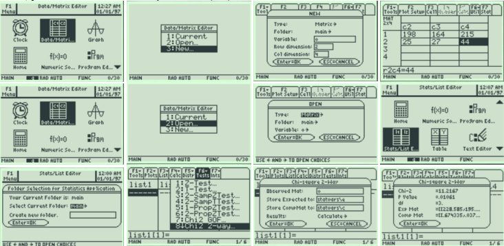If you go back to the matrix menu, you will see some of the expected and $open parenthesis o minus e close parenthesis squared / e$ values.

Sequence of TI-89 screens for the two-way chi-square test: creating a new 2 by 4 matrix named o in the Data/Matrix Editor, entering the observed counts, then in the Stats/List Editor choosing Tests and Chi2 2-way with Observed Mat o and stored expmat and compmat matrices, ending with results Chi-2 = 11.2167, P Value = .01061, df = 3.

To see all the expected values, select [APPS] and select Data/Matrix Editor. Select 2:Open, change the Type to Matrix, change the Folder to statvars, and change the Variable to expmat.

Four TI-89 screens opening the stored expected matrix: the Apps screen with Data/Matrix Editor selected, the 2:Open option, the Open dialog with Type Matrix, Folder statvars, and Variable expmat, and the matrix of expected values with row 1 starting 228.58, 195.3, 167.28 and row 2 starting 32.415, 27.696, 23.722.

To see all the $open parenthesis o minus e close parenthesis squared / e$ values, select [APPS] and select Data/Matrix Editor. Select 2:Open, change the Type to Matrix, change the Folder to statvars, and change the Variable to compmat.

Four TI-89 screens opening the stored comp matrix: the Apps screen with Data/Matrix Editor selected, the 2:Open option, the Open dialog with Folder statvars and Variable compmat, and the matrix of (O−E)²/E values with row 1 starting .67434, .03721, .06425 and row 2 starting 4.7552, .26242, .45308.

If you need to delete a row or column, move the cursor to the row or column that you want to delete, then select F6 Util, then 2:Delete, then choose row or column, then enter. To add a row or column, just arrow over to the new row or column and type in the observed values.

Two TI-89 Data/Matrix Editor screens of the Util menu, with options including 1:Insert, 2:Delete, Sort Column, and 6:Resize Matrix; the Delete submenu offers choices including row and column.

Example 2

The sample data below show the number of companies providing dental insurance for small, medium and large companies. Test to see if there is a relationship between dental insurance coverage and company size. Use $α equals 0.05$ .

Show solution

State the hypotheses.

$H sub 0:$ Dental insurance coverage and company size are independent.

$H sub 1:$ Dental insurance coverage and company size are dependent.

Compute the expected values by taking each row total times column total, divided by grand total.

For the small companies with dental insurance: $(65 \cdot 67) / 160 = 27.21875$ ,

small companies without dental insurance: $(95 \cdot 67) / 160 = 39.78125$ ,

medium companies with dental insurance: $(65 \cdot 64) / 160 = 26$ , etc. See table below.

Compute the test statistic.

Test statistic is $χ^{2} = \sum \frac{(O - E)^{2}}{E} = 1.42082 + 0.03846 + 4.42316 + 0.97214 + 0.02632 + 3.02637 = 9.9073$ .

Use technology to find the p-value using the chi-square cdf with $df = (R - 1) (C - 1) = (2 - 1) (3 - 1) = 2$ .

Using the TI-Calculator, we find the p-value = 0.0071.

The p-value is less than $α$ ; therefore, reject $H sub 0$ .

There is enough evidence to support the claim that there is a relationship between dental insurance coverage and company size.

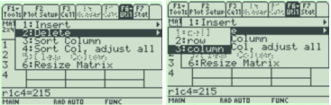
Adapted from Mostly Harmless Statistics by Rachel Webb (Portland State University), hosted on LibreTexts (stats.libretexts.org) and licensed under CC BY-SA 4.0. Changes were made. License: CC-BY-SA-4.0.