10.1 Chi-Square Distribution

A $χ^{2}$ -distribution (chi-square, pronounced “ki-square”) is another special type of distribution for a continuous random variable. The sampling distribution for a variance and standard deviation follows a chi-square distribution.

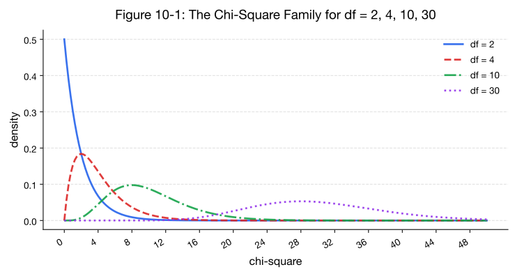
# Figure 10-1: the chi-square family for df = 2, 4, 10, 30
curve(dchisq(x, 2), 0, 50, ylim = c(0, 0.5), xlab = "chi-square", ylab = "density")
curve(dchisq(x, 4),  add = TRUE, col = 2)
curve(dchisq(x, 10), add = TRUE, col = 3)
curve(dchisq(x, 30), add = TRUE, col = 4)   # mean = df, so the peak walks right
legend("topright", c("df=2", "df=4", "df=10", "df=30"), col = 1:4, lwd = 1)
# Every curve starts at zero and is skewed right. Raise a df above 50 and re-run:
# the skew disappears and the curve becomes normal, exactly as property 4 says.

Properties of the $χ^{2}$ -distribution density curve:

Right skewed starting at zero.
The center and spread of a $χ^{2}$ -distribution are determined by the degrees of freedom with a mean = df and standard deviation = $\sqrt{2df}$.
Chi-square variables cannot be negative.
As the degrees of freedom increase, the $χ^{2}$ -distribution becomes normally distributed for df > 50. Figure 10-1 shows $χ^{2}$ -distributions for df of 2, 4, 10, and 30.
The total area under the curve is equal to 1, or 100%.

Chi-square distribution curves for df = 2 (green), 4 (magenta), 10 (gray), and 30 (blue) on one set of axes; the df = 2 curve falls steeply from the left, and as the degrees of freedom increase the curves become lower, more spread out, and more symmetric. — Figure 10-1

We will use the $χ^{2}$ -distribution for hypothesis testing later in this chapter. For now, we are just learning how to find a critical value $χ_{α}^{2}$ .

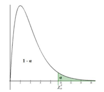
The symbol $χ_{α}^{2}$ is the critical value on the $χ^{2}$ -distribution curve with area 1 – $α$ below the critical value and area $α$ above the critical value, as shown below in Figure 10-2.

Right-skewed chi-square distribution curve with the body labeled 1 − α and the right tail shaded green and labeled α; the boundary between them on the axis is the critical value χ²α. — Figure 10-2

Use technology to compute the critical value for the $χ^{2}$ -distribution.

TI-84: Use the INVCHI2 program downloaded at Rachel Webb’s website: http://MostlyHarmlessStatistics.com. Start the program and enter the area $α$ and the df when prompted.

TI-89: Go to the [Apps] Stat/List Editor, then select F5 [DISTR]. This will get you a menu of probability distributions. Arrow down to Inverse > Inverse Chi-Square and press [ENTER]. Enter the area 1 – $α$ to the left of the $χ$ value and the df into each cell. Press [ENTER].

Excel: =CHISQ.INV(1 – $α$ , df) or =CHISQ.INV.RT( $α$ , df)

Alternatively, use the following online calculator: https://homepage.divms.uiowa.edu/~mbognar/applets/chisq.html.

Example 1

Compute the critical value $χ_{α}^{2}$ for a $α$ = 0.05 and df = 6.

Show solution

Start by drawing the curve and determining the area in the right-tail as shown in Figure 10-3. Then use technology to find the critical value.

Figure 10-3

In Excel there are two options. Use =CHISQ.INV(area in left-tail,df) or right-tail =CHISQ.INV.RT(area in right-tail,df). For this example, then we would have $χ_{α}^{2}$ =CHISQ.INV(0.95,6) or =CHISQ.INV.RT(0.05,6) = 12.5916.

TI-89 use Distr > Inverse Chi-square with area 0.95 and df = 6

Adapted from Mostly Harmless Statistics by Rachel Webb (Portland State University), hosted on LibreTexts (stats.libretexts.org) and licensed under CC BY-SA 4.0. Changes were made. License: CC-BY-SA-4.0.