5.3 Solving Equations with the Properties of Equality

Solving Equations with the Properties of Equality

A source-bound narrated opening with a worked example, an eight-second thinking pause, a checked result, English captions, and a transcript.

Read the transcript Download the video Narration credits and licences

Solve Equations Using the Division and Multiplication Properties of Equality

In an equation of the form $x + a = b$ or $x - a = b$ , we isolate the variable by adding or subtracting the constant term on the side of the equation with the variable. Now we will see how to solve equations that have a variable multiplied by a constant and so will require division to isolate the variable.

Let’s look at a puzzle with envelopes and counters in Figure 5.1.

This image illustrates a workspace divided into two sides. The content of the left side is equal to the content of the right side. On the left side, there are two envelopes each containing an unknown but equal number of counters. On the right side are six counters. — **Figure 5.1** The illustration shows a model of an equation with one variable multiplied by a constant. On the left side of the workspace are two instances of the unknown (envelope), while on the right side of the workspace are six counters.

In the illustration there are two identical envelopes that contain the same number of counters. The left side of the workspace must equal the right side, but the counters on the left side are “hidden” in the envelopes. So how many counters are in each envelope?

How do we determine the number? We have to separate the counters on the right side into two groups of the same size to correspond with the two envelopes on the left side. The 6 counters divided into 2 equal groups gives 3 counters in each group (since $6 \div 2 = 3$ ).

What equation models the situation shown in Figure 5.2? There are two envelopes, and each contains $x$ counters. Together, the two envelopes must contain a total of 6 counters.


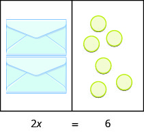
If we divide both sides of the equation by 2, as we did with the envelopes and counters,
we get:

We found that each envelope contains 3 counters. Does this check? We know $2 \cdot 3 = 6$ , so it works! Three counters in each of two envelopes does equal six!

This example leads to the Division Property of Equality.

The goal in solving an equation is to ‘undo’ the operation on the variable. In the next example, the variable is multiplied by 5, so we will divide both sides by 5 to ‘undo’ the multiplication.

Consider the equation $\frac{x}{4} = 3$ . We want to know what number divided by 4 gives 3. So to “undo” the division, we will need to multiply by 4. The Multiplication Property of Equality will allow us to do this. This property says that if we start with two equal quantities and multiply both by the same number, the results are equal.

In the next example, all the variable terms are on the right side of the equation. As always, our goal in solving the equation is to isolate the variable.

Solve Equations That Require Simplification

Many equations start out more complicated than the ones we have been working with.

With these more complicated equations the first step is to simplify both sides of the equation as much as possible. This usually involves combining like terms or using the distributive property.

There are four properties of equality—subtraction, addition, division, and multiplication. We’ll list them all together here for easy reference.

Practice Makes Perfect

Solve Equations Using the Division and Multiplication Properties of Equality

In the following exercises, solve each equation using the Division and Multiplication Properties of Equality and check the solution.

$8 x equals 56$

Show solution

$x equals 7$

$7 p equals 63$

$−5 c equals 55$

Show solution

$c equals −11$

$−9 x equals −27$

$−809 equals 15 y$

Show solution

$y = - \frac{809}{15}$

$−731 equals 19 y$

$−37 p equals −541$

Show solution

$p = \frac{541}{37}$

$−19 m equals −586$

$0.25 z equals 3.25$

Show solution

$z equals 13$

$0.75 a equals 11.25$

$−13 x equals 0$

Show solution

$x equals 0$

$24 x equals 0$

$\frac{x}{4} = 35$

Show solution

$x equals 140$

$\frac{z}{2} = 54$

$−20 = \frac{q}{−5}$

Show solution

$q equals 100$

$\frac{c}{−3} = −12$

$\frac{y}{9} = −16$

Show solution

$y equals −144$

$\frac{q}{6} = −38$

$\frac{m}{−12} = 45$

Show solution

$m equals −540$

$−24 = \frac{p}{−20}$

$− y equals 6$

Show solution

$y equals −6$

$− u equals 15$

$− v equals −72$

Show solution

$v equals 72$

$− x equals −39$

$\frac{2}{3} y = 48$

Show solution

$y equals 72$

$\frac{3}{5} r = 75$

$- \frac{5}{8} w = 40$

Show solution

$w equals −64$

$24 = - \frac{3}{4} x$

$- \frac{2}{5} = \frac{1}{10} a$

Show solution

$a equals −4$

$- \frac{1}{3} q = - \frac{5}{6}$

$- \frac{7}{10} x = - \frac{14}{3}$

Show solution

$x = \frac{20}{3}$

$\frac{3}{8} y = - \frac{1}{4}$

$\frac{7}{12} = - \frac{3}{4} p$

Show solution

$p = - \frac{7}{9}$

$\frac{11}{18} = - \frac{5}{6} q$

$- \frac{5}{18} = - \frac{10}{9} u$

Show solution

$u = \frac{1}{4}$

$- \frac{7}{20} = - \frac{7}{4} v$

Solve Equations That Require Simplification

In the following exercises, solve each equation requiring simplification.

$100 - 16 = 4 p - 10 p - p$

Show solution

$p equals −12$

$−18 - 7 = 5 t - 9 t - 6 t$

$\frac{7}{8} n - \frac{3}{4} n = 9 + 2$

Show solution

$n equals 88$

$\frac{5}{12} q + \frac{1}{2} q = 25 - 3$

$0.25 d + 0.10 d = 6 - 0.75$

Show solution

$d equals 15$

$0.05 p - 0.01 p = 2 + 0.24$

$−10 (q - 4) - 57 = 93$

Show solution

$q equals −11$

$−12 (d - 5) - 29 = 43$

$−10 (x + 4) - 19 = 85$

Show solution

$x = - \frac{72}{5}$

$−15 (z + 9) - 11 = 75$

Corequisite Skills for Introductory Statistics is a custom course edition compiled for Introductory Statistics corequisite courses from OpenStax Contemporary Mathematics, Elementary Algebra 2e, Intermediate Algebra 2e, Prealgebra 2e. Content by OpenStax is reproduced as published, apart from any corrections recorded for this edition. Sections are renumbered to follow the course outline. The course outline is adapted from Larry Green's Support Course for Elementary Statistics (LibreTexts, https://stats.libretexts.org/Bookshelves/Introductory_Statistics/Support_Course_for_Elementary_Statistics), used under CC BY 4.0 (https://creativecommons.org/licenses/by/4.0/). Lessons 2.4 and 6.7 are written for this edition by XYZ Homework. Every OpenStax lesson is abridged to the subsections and practice exercises this course uses. Lessons are headed with their course titles, not the source section titles. Access the complete originals free at openstax.org. License: CC-BY-NC-SA-4.0.