3.7 Multiple Eigenvalues

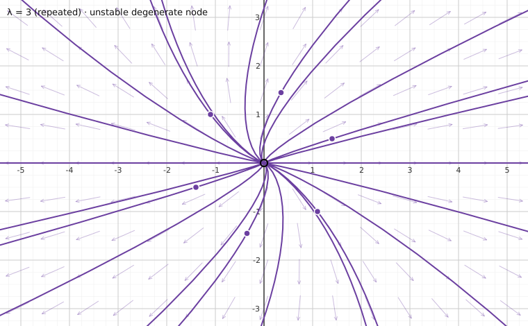
It may very well happen that a matrix has some “repeated” eigenvalues. That is, the characteristic equation $det (A - λ I) = 0$ may have repeated roots. As we have said before, this is actually unlikely to happen for a random matrix. If we take a small perturbation of $A$ (we change the entries of $A$ slightly), then we will get a matrix with distinct eigenvalues. As any system we will want to solve in practice is an approximation to reality anyway, it is not indispensable to know how to solve these corner cases. On the other hand, these cases do come up in applications from time to time. Furthermore, if we have distinct but very close eigenvalues, the behavior is similar to that of repeated eigenvalues, and so understanding that case will give us insight into what is going on.

Function graph showing the phase portrait of x′ = Ax for A = [[3, 1], [0, 3+p]], where the repeated eigenvalue is 3; the origin is an unstable degenerate node. Adjustable parameter: Perturbation of the lower-right entry (eigenvalues 3 and 3 + p) (p) = 0. Viewing window: x from -5.43 to 5.43, y from -3.36 to 3.36. — Lebl works out the defective matrix A = [[3, 1], [0, 3]] later in this section; here its lower-right entry carries a slider, so the eigenvalues are 3 and 3 + p. At p = 0 the matrix is defective: there is a single eigendirection, [1, 0], and every trajectory turns onto it. Nudge p to 0.1 and there are genuinely two eigendirections, [1, 0] and [1, 0.1] — yet the portrait barely changes, which is exactly this paragraph's second claim. Keep dragging and the two directions separate into an ordinary node. At p = −3 the second eigenvalue is 0 and the equilibria fill a whole line through the origin; below that the portrait becomes a saddle.

Geometric Multiplicity

Take the diagonal matrix

$A equals [ 3, 0; 0, 3 ]$

$A$ has an eigenvalue $3$ of multiplicity $2$ . We call the multiplicity of the eigenvalue in the characteristic equation the algebraic multiplicity. In this case, there also exist $2$ linearly independent eigenvectors, $[ 1; 0 ]$ and $[ 0; 1 ]$ corresponding to the eigenvalue $3$ . This means that the so-called geometric multiplicity of this eigenvalue is also $2$ .

In all the theorems where we required a matrix to have $n$ distinct eigenvalues, we only really needed to have $n$ linearly independent eigenvectors. For example, $\vec{x} = A \vec{x}$ has the general solution

$\vec{x} = c_{1} [\begin{matrix} 1 \\ 0 \end{matrix}] e^{3 t} + c_{2} [\begin{matrix} 0 \\ 1 \end{matrix}] e^{3 t} .$

Let us restate the theorem about real eigenvalues. In the following theorem we will repeat eigenvalues according to (algebraic) multiplicity. So for the above matrix $A$ , we would say that it has eigenvalues $3$ and $3$ .

Note

Take $\vec{x} = P \vec{x}$ . Suppose the matrix P is $n \times n$ , has n real eigenvalues (not necessarily distinct), $λ sub 1, ⋯, λ sub n$ and there are $n$ linearly independent corresponding eigenvectors $v sub 1 →, ⋯, v sub n →$ . Then the general solution to ${\vec{x}}^{'} = P \vec{x}$ can be written as:

$\vec{x} = c_{1} \vec{v_{1}} e^{λ_{1} t} + c_{2} \vec{v_{2}} e^{λ_{2} t} + \cdot + c_{n} \vec{v_{n}} e^{λ_{n} t}$

The geometric multiplicity of an eigenvalue of algebraic multiplicity n is equal to the number of corresponding linearly independent eigenvectors. The geometric multiplicity is always less than or equal to the algebraic multiplicity. We have handled the case when these two multiplicities are equal. If the geometric multiplicity is equal to the algebraic multiplicity, then we say the eigenvalue is complete.

In other words, the hypothesis of the theorem could be stated as saying that if all the eigenvalues of $P$ are complete, then there are $n$ linearly independent eigenvectors and thus we have the given general solution.

If the geometric multiplicity of an eigenvalue is $2$ or greater, then the set of linearly independent eigenvectors is not unique up to multiples as it was before. For example, for the diagonal matrix $A equals [ 3, 0; 0, 3 ]$ we could also pick eigenvectors $[ 1; 1 ]$ and $[ 1; minus 1 ]$ , or in fact any pair of two linearly independent vectors. The number of linearly independent eigenvectors corresponding to $λ$ is the number of free variables we obtain when solving $A \vec{v} = λ \vec{v}$ . We pick specific values for those free variables to obtain eigenvectors. If you pick different values, you may get different eigenvectors.

Defective Eigenvalues

If an $n \times n$ matrix has less than n linearly independent eigenvectors, it is said to be deficient. Then there is at least one eigenvalue with an algebraic multiplicity that is higher than its geometric multiplicity. We call this eigenvalue defective and the difference between the two multiplicities we call the defect.

Example 1

The matrix

$[ 3, 1; 0, 3 ]$

has an eigenvalue 3 of algebraic multiplicity 2. Let us try to compute eigenvectors.

$[ 0, 1; 0, 0 ] [ v sub 1; v sub 2 ] equals 0 →$

Show solution

We must have that $v sub 2 equals 0$ . Hence any eigenvector is of the form $[ v sub 1; 0 ]$ . Any two such vectors are linearly dependent, and hence the geometric multiplicity of the eigenvalue is 1. Therefore, the defect is 1, and we can no longer apply the eigenvalue method directly to a system of ODEs with such a coefficient matrix.

Roughly, the key observation is that if $λ$ is an eigenvalue of $A$ of algebraic multiplicity $m$ , then we can find certain $m$ linearly independent vectors solving $(A - λ I)^{k} \vec{v} = \vec{0}$ for various powers $k$ . We will call these generalized eigenvectors.

Let us continue with the example $A equals [ 3, 1; 0, 3 ]$ and the equation $\vec{x} = A \vec{x}$ . We have an eigenvalue $λ equals 3$ of (algebraic) multiplicity 2 and defect 1. We have found one eigenvector $v sub 1 → equals [ 1; 0 ]$ . We have the solution

$1; 0$

We are now stuck, we get no other solutions from standard eigenvectors. But we need two linearly independent solutions to find the general solution of the equation.

In this case, let us try (in the spirit of repeated roots of the characteristic equation for a single equation) another solution of the form

$\vec{x_{2}} = (\vec{v_{2}} + \vec{v_{1}} t) e^{3 t}$

We differentiate to get

${\vec{x}}_{2}^{'} = {\vec{v}}_{1} e^{3 t} + 3 ({\vec{v}}_{2} + {\vec{v}}_{1} t) e^{3 t} = (3 {\vec{v}}_{2} + {\vec{v}}_{1}) e^{3 t} + 3 {\vec{v}}_{1} t e^{3 t} .$

As we are assuming that $x → sub 2$ is a solution, $x → sub 2 prime$ must equal $A x → sub 2$ . So let’s compute $A x → sub 2$ :

$A {\vec{x}}_{2} = A ({\vec{v}}_{2} + {\vec{v}}_{1} t) e^{3 t} = A {\vec{v}}_{2} e^{3 t} + A {\vec{v}}_{1} t e^{3 t} .$

By looking at the coefficients of $e to the power 3 t$ and $t e to the power 3 t$ we see $3 {\vec{v}}_{2} + {\vec{v}}_{1} = A {\vec{v}}_{2}$ and $3 v → sub 1 equals A v → sub 1$ . This means that

$(A - 3 I) {\vec{v}}_{2} = {\vec{v}}_{1}, and (A - 3 I) {\vec{v}}_{1} = \vec{0} .$

Therefore, $x → sub 2$ is a solution if these two equations are satisfied. The second equation is satisfied if $v → sub 1$ is an eigenvector, and we found the eigenvector above, so let $v → sub 1 equals [ 1; 0 ]$ . So, if we can find a $v → sub 2$ that solves $(A - 3 I) {\vec{v}}_{2} = {\vec{v}}_{1}$ , then we are done. This is just a bunch of linear equations to solve and we are by now very good at that. Let us solve $(A - 3 I) {\vec{v}}_{2} = {\vec{v}}_{1}$ . Write

$[ 0, 1; 0, 0 ] [ a; b ] equals [ 1; 0 ].$

By inspection we see that letting $a equals 0$ ( $a$ could be anything in fact) and $b equals 1$ does the job. Hence we can take $v → sub 2 equals [ 0; 1 ]$ . Our general solution to ${\vec{x}}^{'} = A \vec{x}$ is

$\vec{x} = c_{1} [\begin{matrix} 1 \\ 0 \end{matrix}] e^{3 t} + c_{2} ([\begin{matrix} 0 \\ 1 \end{matrix}] + [\begin{matrix} 1 \\ 0 \end{matrix}] t) e^{3 t} = [\begin{matrix} c_{1} e^{3 t} + c_{2} t e^{3 t} \\ c_{2} e^{3 t} \end{matrix}] .$

Let us check that we really do have the solution. First $x_{1}^{'} = c_{1} 3 e^{3 t} + c_{2} e^{3 t} + 3 c_{2} t e^{3 t} = 3 x_{1} + x_{2}$ . Good. Now $x_{2}^{'} = 3 c_{2} e^{3 t} = 3 x_{2}$ . Good.

Note that the system ${\vec{x}}^{'} = A \vec{x}$ has a simpler solution since $A$ is a so-called upper triangular matrix, that is every entry below the diagonal is zero. In particular, the equation for $x sub 2$ does not depend on $x sub 1$ . Mind you, not every defective matrix is triangular.

Let us describe the general algorithm. Suppose that $λ$ is an eigenvalue of multiplicity $2$ , defect $1$ . First find an eigenvector $v sub 1 →$ of $λ$ . Then, find a vector $v sub 2 →$ such that

$(A - λ I) \vec{v_{2}} = \vec{v_{1}}$

This gives us two linearly independent solutions

$\begin{matrix} \vec{x_{1}} = \vec{v_{1}} e^{λ t} \\ \vec{x_{2}} = (\vec{v_{2}} + \vec{v_{1}} t) e^{λ t} \end{matrix}$

Example 2

Consider the system

${\vec{x}}^{'} = [\begin{matrix} 2 & - 5 & 0 \\ 0 & 2 & 0 \\ - 1 & 4 & 1 \end{matrix}] \vec{x} .$

Compute the eigenvalues,

Show solution

$0 = det (A - λ I) = det ([\begin{matrix} 2 - λ & - 5 & 0 \\ 0 & 2 - λ & 0 \\ - 1 & 4 & 1 - λ \end{matrix}]) = (2 - λ)^{2} (1 - λ) .$

The eigenvalues are 1 and 2, where 2 has multiplicity 2. We leave it to the reader to find that

[ 0; 0; 1 ]

is an eigenvector for the eigenvalue

λ equals 1

Let’s focus on $λ equals 2$ . We compute eigenvectors:

$\vec{0} = (A - 2 I) \vec{v} = [\begin{matrix} 0 & - 5 & 0 \\ 0 & 0 & 0 \\ - 1 & 4 & - 1 \end{matrix}] [\begin{matrix} v_{1} \\ v_{2} \\ v_{3} \end{matrix}] .$

The first equation says that

v sub 2 equals 0

, so the last equation is

- v_{1} - v_{3} = 0

. Let

v sub 3

be the free variable to find that

v_{1} = - v_{3}

. Perhaps let

v_{3} = - 1

to find an eigenvector

[ 1; 0; minus 1 ]

. Problem is that setting

v sub 3

to anything else just gets multiples of this vector and so we have a defect of 1. Let

v → sub 1

be the eigenvector and let’s look for a generalized eigenvector

v → sub 2

$(A - 2 I) {\vec{v}}_{2} = {\vec{v}}_{1},$

$[\begin{matrix} 0 & - 5 & 0 \\ 0 & 0 & 0 \\ - 1 & 4 & - 1 \end{matrix}] [\begin{matrix} a \\ b \\ c \end{matrix}] = [\begin{matrix} 1 \\ 0 \\ - 1 \end{matrix}],$

where we used

a

b

c

as components of

v → sub 2

for simplicity. The first equation says

- 5 b = 1

b = \frac{- 1}{5}

. The second equation says nothing. The last equation is

- a + 4 b - c = - 1

, or

a + \frac{4}{5} + c = 1

, or

a + c = \frac{1}{5}

. We let

c

be the free variable and we choose

c equals 0

. We find

{\vec{v}}_{2} = [\begin{matrix} \frac{1}{5} \\ \frac{- 1}{5} \\ 0 \end{matrix}]

The general solution is therefore,

$\vec{x} = c_{1} [\begin{matrix} 0 \\ 0 \\ 1 \end{matrix}] e^{t} + c_{2} [\begin{matrix} 1 \\ 0 \\ - 1 \end{matrix}] e^{2 t} + c_{3} ([\begin{matrix} \frac{1}{5} \\ \frac{- 1}{5} \\ 0 \end{matrix}] + [\begin{matrix} 1 \\ 0 \\ - 1 \end{matrix}] t) e^{2 t} .$

This machinery can also be generalized to higher multiplicities and higher defects. We will not go over this method in detail, but let us just sketch the ideas. Suppose that $A$ has an eigenvalue $λ$ of multiplicity $m$ . We find vectors such that

$(A - λ I)^{k} \vec{(} v) = \vec{(} 0), but (A - λ I)^{k - 1} \vec{v} \neq \vec{0}$

Such vectors are called generalized eigenvectors (then $\vec{v_{1}} = (A - λ I)^{k - 1} \vec{v}$ is an eigenvector). For every eigenvector $v → sub 1$ we find a chain of generalized eigenvectors $v → sub 2$ through ${\vec{v}}_{k}$ such that:

$\begin{matrix} (A - λ I) \vec{v_{1}} = \vec{0}, \\ (A - λ I) \vec{v_{2}} = \vec{v_{1}}, \\ ⋮ \\ (A - λ I) \vec{v_{k}} = \vec{v_{k - 1}} . \end{matrix}$

Really once you find the ${\vec{v}}_{k}$ such that ${(A - λ I)}^{k} {\vec{v}}_{k} = \vec{0}$ but ${(A - λ I)}^{k - 1} {\vec{v}}_{k} ⧸ = \vec{0}$ , you find the entire chain since you can compute the rest, ${\vec{v}}_{k - 1} = (A - λ I) {\vec{v}}_{k}$ , ${\vec{v}}_{k - 2} = (A - λ I) {\vec{v}}_{k - 1}$ , etc. We form the linearly independent solutions

$\begin{matrix} \vec{x_{1}} = \vec{v_{1}} e^{λ t} \\ \vec{x_{2}} = (\vec{v_{2}} + \vec{v_{1}} t) e^{λ t} \\ ⋮ \\ \vec{x_{k}} = (\vec{v_{k}} + {\vec{v}}_{k - 1} t + {\vec{v}}_{k - 2} \frac{t^{2}}{2} + \dots + {\vec{v}}_{2} \frac{t^{k - 2}}{(k - 2)!} + {\vec{v}}_{1} \frac{t^{k - 1}}{(k - 1)!}) e^{λ t}) \end{matrix}$

Recall that $k! = 1 \cdot 2 \cdot 3 \dots (k - 1) \cdot k$ is the factorial. If you have an eigenvalue of geometric multiplicity $ℓ$ , you will have to find $ℓ$ such chains (some of them might be short: just the single eigenvector equation). We go until we form $m$ linearly independent solutions where $m$ is the algebraic multiplicity. We don’t quite know which specific eigenvectors go with which chain, so start by finding ${\vec{v}}_{k}$ first for the longest possible chain and go from there.

For example, if $λ$ is an eigenvalue of $A$ of algebraic multiplicity $3$ and defect $2$ , then solve

$(A - λ I) {\vec{v}}_{1} = \vec{0}, (A - λ I) {\vec{v}}_{2} = {\vec{v}}_{1}, (A - λ I) {\vec{v}}_{3} = {\vec{v}}_{2} .$

That is, find

v → sub 3

such that

{(A - λ I)}^{3} {\vec{v}}_{3} = \vec{0}

, but

{(A - λ I)}^{2} {\vec{v}}_{3} ⧸ = \vec{0}

. Then you are done as

{\vec{v}}_{2} = (A - λ I) {\vec{v}}_{3}

and

{\vec{v}}_{1} = (A - λ I) {\vec{v}}_{2}

. The 3 linearly independent solutions are

${\vec{x}}_{1} = {\vec{v}}_{1} e^{λ t}, {\vec{x}}_{2} = ({\vec{v}}_{2} + {\vec{v}}_{1} t) e^{λ t}, {\vec{x}}_{3} = ({\vec{v}}_{3} + {\vec{v}}_{2} t + {\vec{v}}_{1} \frac{t^{2}}{2}) e^{λ t} .$

If on the other hand $A$ has an eigenvalue $λ$ of algebraic multiplicity $3$ and defect $1$ , then solve

$(A - λ I) {\vec{v}}_{1} = \vec{0}, (A - λ I) {\vec{v}}_{2} = \vec{0}, (A - λ I) {\vec{v}}_{3} = {\vec{v}}_{2} .$

Here

v → sub 1

and

v → sub 2

are actual honest eigenvectors, and

v → sub 3

is a generalized eigenvector. So there are two chains. To solve, first find a

v → sub 3

such that

{(A - λ I)}^{2} {\vec{v}}_{3} = \vec{0}

, but

(A - λ I) {\vec{v}}_{3} ⧸ = \vec{0}

. Then

{\vec{v}}_{2} = (A - λ I) {\vec{v}}_{3}

is going to be an eigenvector. Then solve for an eigenvector

v → sub 1

that is linearly independent from

v → sub 2

. You get 3 linearly independent solutions

${\vec{x}}_{1} = {\vec{v}}_{1} e^{λ t}, {\vec{x}}_{2} = {\vec{v}}_{2} e^{λ t}, {\vec{x}}_{3} = ({\vec{v}}_{3} + {\vec{v}}_{2} t) e^{λ t} .$

Adapted from Differential Equations for Engineers by Jiří Lebl (Oklahoma State University), hosted on LibreTexts (math.libretexts.org) and licensed under CC BY-SA 4.0. Changes were made. License: CC-BY-SA-4.0.