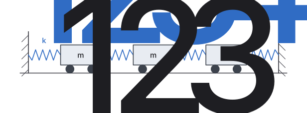
While we did say that we will usually only look at first order systems, it is sometimes more convenient to study the system in the way it arises naturally. For example, suppose we have 3 masses connected by springs between two walls. We could pick any higher number, and the math would be essentially the same, but for simplicity we pick 3 right now. Let us also assume no friction, that is, the system is undamped. The masses are , and and the spring constants are , and . Let be the displacement from rest position of the first mass, and and the displacement of the second and third mass. We will make, as usual, positive values go right (as grows, the first mass is moving right). See Figure .
Figure : System of masses and springs.
This simple system turns up in unexpected places. For example, our world really consists of many small particles of matter interacting together. When we try the above system with many more masses, we obtain a good approximation to how an elastic material behaves. By somehow taking a limit of the number of masses going to infinity, we obtain the continuous one dimensional wave equation (that we study in Section 4.7). But we digress.
Let us set up the equations for the three mass system. By Hooke’s law we have that the force acting on the mass equals the spring compression times the spring constant. By Newton’s second law we have that force is mass times acceleration. So if we sum the forces acting on each mass and put the right sign in front of each term, depending on the direction in which it is acting, we end up with the desired system of equations.
We define the matrices
We write the equation simply as
At this point we could introduce 3 new variables and write out a system of 6 first order equations. We claim this simple setup is easier to handle as a second order system. We call the displacement vector, the mass matrix, and the stiffness matrix.
As with a single equation we want to “divide by .” This means computing the inverse of . The masses are all nonzero and is a diagonal matrix, so comping the inverse is easy:
This fact follows readily by how we multiply diagonal matrices. As an exercise, you should verify that
Let . We look at the system , or
Many real world systems can be modeled by this equation. For simplicity, we will only talk about the given masses-and-springs problem. We try a solution of the form
We compute that for this guess, We plug our guess into the equation and get
We divide by to arrive at . Hence if is an eigenvalue of and is a corresponding eigenvector, we have found a solution.
In our example, and in other common applications, has only real negative eigenvalues (and possibly a zero eigenvalue). So we study only this case. When an eigenvalue is negative, it means that is negative. Hence there is some real number such that . Then . The solution we guessed was
By taking the real and imaginary parts (note that is real), we find that and are linearly independent solutions.
If an eigenvalue is zero, it turns out that both and are solutions, where is an eigenvector corresponding to the eigenvalue 0.
We use this solution and the setup from the introduction of this section even when some of the masses and springs are missing. For example, when there are only 2 masses and only 2 springs, simply take only the equations for the two masses and set all the spring constants for the springs that are missing to zero.
The first term,
corresponds to the mode where the masses move synchronously in the same direction.
The second term,
corresponds to the mode where the masses move synchronously but in opposite directions.
The general solution is a combination of the two modes. That is, the initial conditions determine the amplitude and phase shift of each mode. As an example, suppose we have initial conditions
We use the constants to solve for initial conditions. First
We solve (exercise) to find , . To find the and , we differentiate first:
Now we solve:
Again solve (exercise) to find , . So our solution is
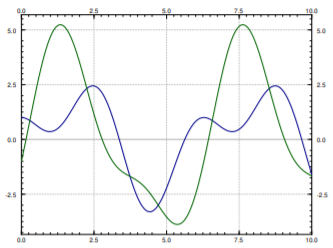
The graphs of the two displacements, and of the two carts is in Figure .
Figure : Superposition of the two modes given the initial conditions.
OK, let us first set the system up. Let be the time when the two cars link up. Let be the displacement of the first car from the position at , and let be the displacement of the second car from its original location. Then the time when is exactly the time when impact with wall occurs. For this is the speed at impact. This system acts just like the system of the previous example but without . Hence the equation is
or
We compute the eigenvalues of . It is not hard to see that the eigenvalues are and (exercise). Furthermore, eigenvectors are and respectively (exercise). Then and by the second part of the theorem we find our general solution to be
We now apply the initial conditions. First the cars start at position so and . The first car is traveling at , so and the second car starts at rest, so . The first conditions says
It is not hard to see that . We set and in and differentiate to get
So
Solving these two equations we find and . Hence the position of our cars is (until the impact with the wall)
Note how the presence of the zero eigenvalue resulted in a term containing . This means that the carts will be traveling in the positive direction as time grows, which is what we expect.
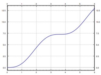
What we are really interested in is the second expression, the one for . We have . See Figure for the plot of versus time.
Figure : Position of the second car in time (ignoring the wall).
Just from the graph we can see that time of impact will be a little more than 5 seconds from time zero. For this we have to solve the equation . Using a computer (or even a graphing calculator) we find that seconds.
As for the speed we note that . At time of impact ( seconds from ) we get that .
The maximum speed is the maximum of , which is . We are traveling at almost the maximum speed when we hit the wall.
Suppose that Bob is a tiny person sitting on car 2. Bob has a Martini in his hand and would like not to spill it. Let us suppose Bob would not spill his Martini when the first car links up with car 2, but if car 2 hits the wall at any speed greater than zero, Bob will spill his drink. Suppose Bob can move car 2 a few meters towards or away from the wall (he cannot go all the way to the wall, nor can he get out of the way of the first car). Is there a “safe” distance for him to be at? A distance such that the impact with the wall is at zero speed?
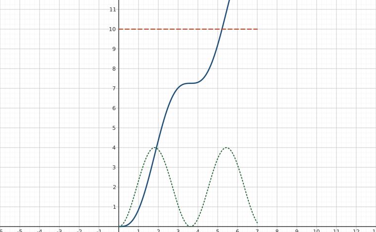
Interactive figureHow far from the wall can Bob keep his Martini?Drag the Distance from car 2 to the wall slider from 5 to 11.
XYZ Graph · viewer build 5edf91b
Car 2's position x₂(t) = 2t − (2/√3)·sin(√3·t) (solid), the wall as a movable line at distance d (dashed), and the impact speed x₂′(t) = 2 − 2·cos(√3·t) (dotted); the horizontal axis is time t in seconds. At Lebl's d = 10 m the wall cuts the curve on a steep stretch — impact at t ≈ 5.22 s, speed ≈ 3.85 m/s. Drag d down and the crossing slides left and flattens until, at d ≈ 7.26 m (= 4π/√3), the line is tangent to the plateau at t = 2π/√3, right where the dotted speed curve touches zero. That tangency is Bob's safe distance; drag past it and the curve steepens again.
The answer is yes. Looking at Figure , we note the “plateau” between and . There is a point where the speed is zero. To find it we need to solve . This is when or in other words when and so on. We plug in the first value to obtain . So a “safe” distance is about 7 and a quarter meters from the wall.
Alternatively Bob could move away from the wall towards the incoming car 2 where another safe distance is and so on, using all the different such that . Of course is always a solution here, corresponding to , but that means standing right at the wall.
Forced Oscillations
Finally we move to forced oscillations. Suppose that now our system is
(3.6.1)
That is, we are adding periodic forcing to the system in the direction of the vector .
As before, this system just requires us to find one particular solution , add it to the general solution of the associated homogeneous system , and we will have the general solution to (3.6.1). Let us suppose that is not one of the natural frequencies of , then we can guess
where is an unknown constant vector. Note that we do not need to use sine since there are only second derivatives. We solve for to find . This is really just the method of undetermined coefficients for systems. Let us differentiate twice to get
We cancel out the cosine and rearrange the equation to obtain
So
Of course this is possible only if is invertible. That matrix is invertible if and only if is not an eigenvalue of . That is true if and only if is not a natural frequency of the system.
We simplified things a little bit. If we wish to have the forcing term to be in the units of force, say Newtons, then we must write
If we then write things in terms of , we have
where .
Note that given force , we write the equation as to get the units right. Then we write . The term in is in units of force per unit mass.
If is a natural frequency of the system resonance occurs because we will have to try a particular solution of the form
That is assuming that the eigenvalues of the coefficient matrix are distinct. Next, note that the amplitude of this solution grows without bound as grows.
These eBooks are a prerelease and are not yet certified conformant with WCAG 2.1 AA or ADA Title II. Every page is built against an automated accessibility gate, and the published editions will meet ADA Title II requirements when they release in late September 2026. If something is unusable, please tell us.