Often we do not have just one dependent variable and just one differential equation, we may end up with systems of several equations and several dependent variables even if we start with a single equation.
If we have several dependent variables, suppose , ,..., , then we can have a differential equation involving all of them and their derivatives. For example, . Usually, when we have two dependent variables we have two equations such as
for some functions and . We call the above a system of differential equations. More precisely, the above is a second order system of ODEs as second order derivatives appear. The system
is a first order system, where are the dependent variables, and is the independent variable.
The terminology for systems is essentially the same as for single equations. For the system above, a solution is a set of three functions , , , such that
We usually also have an initial condition. Just like for single equations we specify , , and for some fixed . For example, , , . For some constants , , and . For the second order system we would also specify the first derivatives at a point. And if we find a solution with constants in it, where by solving for the constants we find a solution for any initial condition, we call this solution the general solution. Best to look at a simple example.
Generally, we will not be so lucky to be able to solve for each variable separately as in the example above, and we will have to solve for all variables at once. While we won’t generally be able to solve for one variable and then the next, we will try to salvage as much as possible from this technique. It will turn out that in a certain sense we will still (try to) solve a bunch of single equations and put their solutions together. Let’s not worry right now about how to solve systems yet.
We will mostly consider the linear systems. The example above is a so-called linear first order system. It is linear as none of the dependent variables or their derivatives appear in nonlinear functions or with powers higher than one (, , and , constants, and functions of can appear, but not or or ). Another, more complicated, example of a linear system is
Applications
Let us consider some simple applications of systems and how to set up the equations.
Changing to First Order
Before we talk about how to handle systems, let us note that in some sense we need only consider first order systems. Let us take an order differential equation
We define new variables and write the system
We solve this system for . Once we have solved for the ’s, we can discard through and let . We note that this solves the original equation.
A similar process can be followed for a system of higher order differential equations. For example, a system of differential equations in unknowns, all of order , can be transformed into a first order system of equations and unknowns.
It is useful to go back and forth between systems and higher order equations for other reasons. For example, software for solving ODE numerically (approximation) is generally for first order systems. To use it, you take whatever ODE you want to solve and convert it to a first order system. It is not very hard to adapt computer code for the Euler or Runge–Kutta method for first order equations to handle first order systems. We simply treat the dependent variable not as a number but as a vector. In many mathematical computer languages there is almost no distinction in syntax.
Autonomous Systems and Vector Fields
A system where the equations do not depend on the independent variable is called an autonomous system. For example the system , is autonomous as is the independent variable but does not appear in the equations.
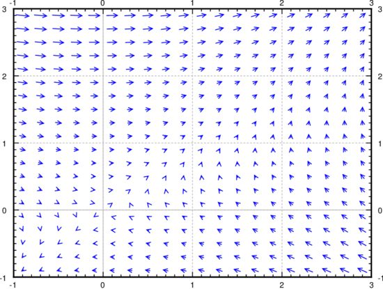
For autonomous systems we can draw the so-called direction field or vector field, a plot similar to a slope field, but instead of giving a slope at each point, we give a direction (and a magnitude). The previous example, , , says that at the point the direction in which we should travel to satisfy the equations should be the direction of the vector with the speed equal to the magnitude of this vector. So we draw the vector at the point and we do this for many points on the -plane. For example, at the point we draw the vector , a vector pointing to the right and a little bit up, while at the point we draw the vector a vector that points straight up. When drawing the vectors, we will scale down their size to fit many of them on the same direction field. If we drew the arrows at the actual size, the diagram would be a jumbled mess once you would draw more than a couple of arrows. So we scale them all so that not even the longest one interferes with the others. We are mostly interested in their direction and relative size. See Figure .
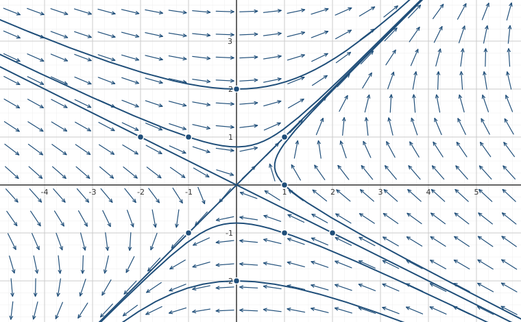
Interactive figureDirection field and trajectories for x' = 2y - x, y' = xDrag the Coefficient of y in x' (Lebl's system is k = 2) slider from -2 to 3.
XYZ Graph · viewer build 5edf91b
This section's own direction field, x′ = 2y − x, y′ = x, carrying nine trajectories instead of the single one Lebl's Figure 4 shows. The curve seeded at (1, 0) is his: follow it two units of t and it arrives at (2.475, 2.457), exactly the value the text computes. Four seeds sit on the two directions the section's own y″ + y′ − 2y = 0 hands you — the e^t part of the solution runs out along (1, 1), the e^(-2t) part runs in along (2, −1) — so those four draw as perfectly straight rays, the skeleton one trajectory cannot show. Now drag k, which stands in for Lebl's 2: the characteristic equation becomes λ² + λ − k = 0, so crossing k = 0 destroys the saddle outright (the whole y-axis turns into equilibria) and leaves a stable node, and below k = −0.25 the discriminant 1 + 4k goes negative and that node becomes a spiral sink — three regimes in one drag.
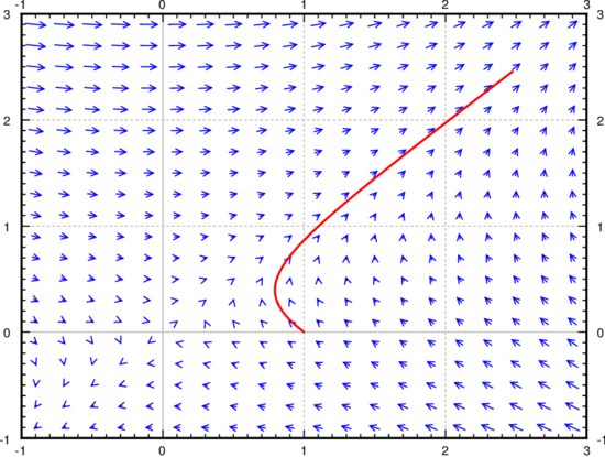
We can draw a path of the solution in the plane. Suppose the solution is given by , . We pick an interval of (say for our example) and plot all the points for in the selected range. The resulting picture is called the phase portrait (or phase plane portrait). The particular curve obtained is called the trajectory or solution curve. See an example plot in Figure . In the figure the solution starts at and travels along the vector field for a distance of 2 units of . We solved this system precisely, so we compute and to find and . This point corresponds to the top right end of the plotted solution curve in the figure.
Notice the similarity to the diagrams we drew for autonomous systems in one dimension. But note how much more complicated things become when we allow just one extra dimension.
We can draw phase portraits and trajectories in the -plane even if the system is not autonomous. In this case, however, we cannot draw the direction field, since the field changes as changes. For each we would get a different direction field.
Figure : The direction field for .Figure : The direction field for with the trajectory of the solution starting at for .
Picard’s theorem
Perhaps before going further, let us mention that Picard’s theorem on existence and uniqueness still holds for systems of ODE. Let us restate this theorem in the setting of systems. A general first order system is of the form
(3.1.1)
That is, a unique solution exists for any initial condition given that the system is reasonable ( and its partial derivatives in the variables are continuous). As for single equations we may not have a solution for all time , but at least for some short period of time.
As we can change any th order ODE into a first order system, then we notice that this theorem provides also the existence and uniqueness of solutions for higher order equations that we have until now not stated explicitly.
These eBooks are a prerelease and are not yet certified conformant with WCAG 2.1 AA or ADA Title II. Every page is built against an automated accessibility gate, and the published editions will meet ADA Title II requirements when they release in late September 2026. If something is unusable, please tell us.