3.5 Two dimensional systems and their vector fields

Let us take a moment to talk about constant coefficient linear homogeneous systems in the plane. Much intuition can be obtained by studying this simple case. Suppose we use coordinates $(x, y)$ for the plane as usual, and suppose $\begin{matrix} a b \\ c d \end{matrix}$ is a $2 times 2$ matrix. Consider the system

$[^{\begin{matrix} x \\ y \end{matrix}]'} = P [\begin{matrix} x \\ y \end{matrix}] or [^{\begin{matrix} x \\ y \end{matrix}]'} = [\begin{matrix} a & b \\ c & d \end{matrix}] [\begin{matrix} x \\ y \end{matrix}] .$

(3.5.1)

The system is autonomous (compare this section to Section 1.6) and so we can draw a vector field (see end of Section 3.1). We will be able to visually tell what the vector field looks like and how the solutions behave, once we find the eigenvalues and eigenvectors of the matrix $P$ . For this section, we assume that $P$ has two eigenvalues and two corresponding eigenvectors.

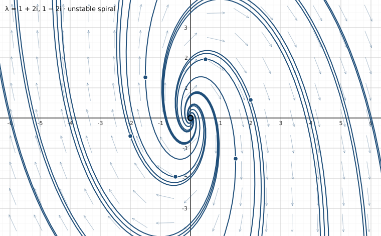
Function graph showing the phase portrait of x′ = Ax for A = [[a, 1], [c, a]], where the eigenvalues are 1 + 2i and 1 − 2i; the origin is an unstable spiral. Adjustable parameters: Diagonal entry a — shifts both eigenvalues (stability) (a) = 1, Lower-left entry c — sign of the discriminant (spiral vs node) (c) = -4. Viewing window: x from -6.33 to 6.33, y from -3.92 to 3.92. — Lebl's summary table lists six behaviors; this one family produces all six. For x′ = Ax with A = [[a, 1], [c, a]] the eigenvalues are exactly λ = a ± √c, so the two sliders are the two things that decide the picture: a shifts both eigenvalues (stability), and the sign of c decides complex versus real. It opens on Lebl's own spiral source [[1, 1], [−4, 1]], λ = 1 ± 2i. Drag c up from −4 and the spiral uncoils into an unstable node as the discriminant passes zero — at c = 0 exactly you get the defective [[a, 1], [0, a]], the shape of §3.7's [[3, 1], [0, 3]]. At c = a² one eigenvalue is 0, the singular case this section's last paragraph sets aside; past it the two real eigenvalues have opposite signs and the node becomes a saddle. Then put c back to −4 and drag a down through 0: spiral source → Lebl's own center [[0, 1], [−4, 0]], λ = ±2i → spiral sink, λ = −1 ± 2i.

1

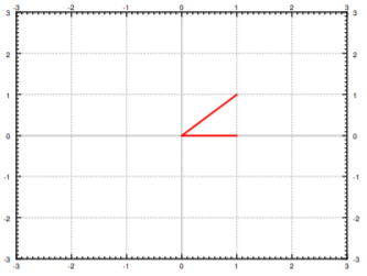
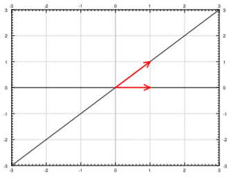
Suppose that the eigenvalues of $P$ are real and positive. We find two corresponding eigenvectors and plot them in the plane. For example, take the matrix $[ 1, 1; 0, 2 ]$ . The eigenvalues are 1 and 2 and corresponding eigenvectors are $[ 1; 0 ]$ and $[ 1; 1 ]$ . See Figure $1$ .

Plot on a grid from -3 to 3 showing only two red eigenvector segments from the origin: one along the 45-degree diagonal to (1, 1), one along the horizontal axis to (1, 0). — Figure $1$ : Eigenvectors of $P$ .

Now suppose that $x$ and $y$ are on the line determined by an eigenvector $\vec{v}$ for an eigenvalue $λ$ . That is, $[ x; y ] equals a v →$ for some scalar $a$ . Then

$[^{\begin{matrix} x \\ y \end{matrix}]'} = P [\begin{matrix} x \\ y \end{matrix}] = P (a \vec{v}) = a (P \vec{v}) = a λ \vec{v}$

The derivative is a multiple of $\vec{v}$ and hence points along the line determined by $\vec{v}$ . As $λ greater than 0$ , the derivative points in the direction of $v e c v$ when $α$ is positive and in the opposite direction when $α$ is negative. Let us draw the lines determined by the eigenvectors, and let us draw arrows on the lines to indicate the directions. See Figure $2$ .

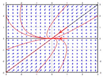
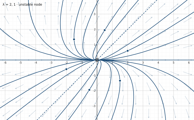
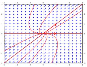
We fill in the rest of the arrows for the vector field and we also draw a few solutions. See Figure $3$ . Notice that the picture looks like a source with arrows coming out from the origin. Hence we call this type of picture a source or sometimes an unstable node.

Plot on a grid from -3 to 3 with the eigenvector lines through the origin drawn in black, the diagonal y equals x and the horizontal axis, and red arrows to (1, 1) and (1, 0) marking direction. — Figure $2$ : Eigenvectors of $P$ with directions.

Vector field of blue arrows on a square from -3 to 3, all pointing away from the origin, with red trajectories running outward along the horizontal axis and the diagonal y equals x: a source. — Figure $3$ : Example source vector field with eigenvectors and solutions.

2

Suppose both eigenvalues were negative. For example, take the negation of the matrix in case 1, $[\begin{matrix} - 1 & - 1 \\ 0 & - 2 \end{matrix}]$ . The eigenvalues are -1 and -2 and corresponding eigenvectors are the same, $[ 1; 0 ]$ and $[ 1; 1 ]$ . The calculation and the picture are almost the same. The only difference is that the eigenvalues are negative and hence all arrows are reversed. We get the picture in Figure $4$ . We call this kind of picture a sink or sometimes a stable node.

Vector field of blue arrows on a square from -3 to 3, all pointing toward the origin, with red trajectories flattening onto the horizontal axis and sliding in without circling: a sink. — Figure $4$ : Example sink vector field with eigenvectors and solutions.

3

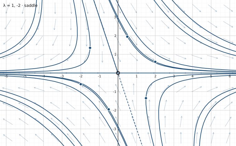
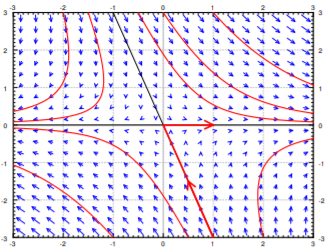
Suppose one eigenvalue is positive and one is negative. For example the matrix $1 1; 0 minus 2$ . The eigenvalues are $1$ and $− 2$ and corresponding eigenvectors are $1; 0$ and $1; minus 3$ .

We reverse the arrows on one line (corresponding to the negative eigenvalue) and we obtain the picture in Figure $5$ . We call this picture a saddle point.

Phase portrait of a saddle on axes from -3 to 3: red trajectories in a blue vector field sweep in along a steep eigenvector line of slope about -3, then out along the horizontal axis. — Figure $5$ : Example saddle vector field with eigenvectors and solutions.

For the next three cases we will assume the eigenvalues are complex. In this case the eigenvectors are also complex and we cannot just plot them in the plane.

4

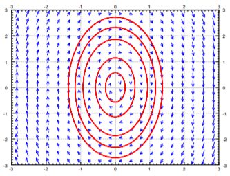
Suppose the eigenvalues are purely imaginary. That is, suppose the eigenvalues are $\pm i b$ . For example, let $P = [\begin{matrix} 0 & 1 \\ - 4 & 0 \end{matrix}]$ . The eigenvalues turn out to be $± 2 i$ and eigenvectors are $[ 1; 2 i ]$ and $[ 1; minus 2 i ]$ . Consider the eigenvalue $2 i$ and its eigenvector $[ 1; 2 i ]$ . The real and imaginary parts of $v → e to the power i 2 t$ are

$R e [\begin{matrix} 1 \\ 2 i \end{matrix}] e^{i 2 t} = [\begin{matrix} c o s (2 t) \\ - 2 s i n (2 t) \end{matrix}], I m [\begin{matrix} 1 \\ 2 i \end{matrix}] e^{i 2 t} = [\begin{matrix} s i n (2 t) \\ 2 c o s (2 t) \end{matrix}]$

We can take any linear combination of them to get other solutions, which one we take depends on the initial conditions. Now note that the real part is a parametric equation for an ellipse. Same with the imaginary part and in fact any linear combination of the two. This is what happens in general when the eigenvalues are purely imaginary. So when the eigenvalues are purely imaginary, we get ellipses for the solutions. This type of picture is sometimes called a center. See Figure $6$ .

Center vector field on axes from -3 to 3: blue arrows circulate clockwise and five nested red loops, taller than wide, close on themselves around the origin. — Figure $6$ : Example center vector field.

5

Now suppose the complex eigenvalues have a positive real part. That is, suppose the eigenvalues are $a \pm i b$ for some $a greater than 0$ . For example, let $P = [\begin{matrix} 1 & 1 \\ - 4 & 1 \end{matrix}]$ . The eigenvalues turn out to be $1 ± 2 i$ and eigenvectors are $[ 1; 2 i ]$ and $[ 1; minus 2 i ]$ . We take $1 ± 2 i$ and its eigenvector $[ 1; 2 i ]$ and find the real and imaginary of $\vec{v} e^{(1 + 2 i) t}$ are

$R e [\begin{matrix} 1 \\ 2 i \end{matrix}] e^{(1 + 2 i) t} = e^{t} [\begin{matrix} c o s (2 t) \\ - 2 s i n (2 t) \end{matrix}] I m [\begin{matrix} 1 \\ 2 i \end{matrix}] e^{(1 + 2 i) t} = e^{t} [\begin{matrix} s i n (2 t) \\ 2 c o s (2 t) \end{matrix}]$

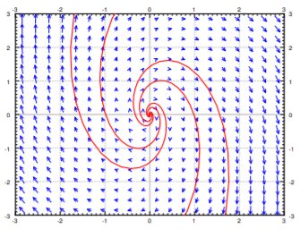
Note the $e^{t}$ in front of the solutions. This means that the solutions grow in magnitude while spinning around the origin. Hence we get a spiral source. See Figure $7$ .

Spiral source vector field on axes from -3 to 3: red curves spiral clockwise outward from the origin, growing steadily, with blue arrows leaning outward everywhere. — Figure $7$ : Example spiral source vector field.

6

Finally suppose the complex eigenvalues have a negative real part. That is, suppose the eigenvalues are $- a \pm i b$ for some $a greater than 0$ . For example, let $P = [\begin{matrix} - 1 & - 1 \\ 4 & - 1 \end{matrix}]$ . The eigenvalues turn out to be $minus 1 ± 2 i$ and eigenvectors are $[ 1; minus 2 i ]$ and $[ 1; 2 i ]$ . We take $- 1 - 2 i$ and its eigenvector $[ 1; 2 i ]$ and find the real and imaginary of $\vec{v} e^{(- 1 - 2 i) t}$ are

$R e [\begin{matrix} 1 \\ 2 i \end{matrix}] e^{(- 1 - 2 i) t} = e^{- t} [\begin{matrix} c o s (2 t) \\ 2 s i n (2 t) \end{matrix}] I m [\begin{matrix} 1 \\ 2 i \end{matrix}] e^{(- 1 - 2 i) t} = e^{- t} [\begin{matrix} - s i n (2 t) \\ 2 c o s (2 t) \end{matrix}]$

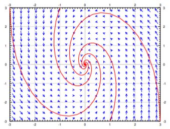
Note the $e^{- t}$ in front of the solutions. This means that the solutions shrink in magnitude while spinning around the origin. Hence we get a spiral sink. See Figure $8$ .

Spiral sink vector field on axes from -3 to 3: red trajectories wind counterclockwise inward from the edges, tightening onto the origin as the blue arrows tilt inward. — Figure $8$ : Example spiral sink vector field.

We summarize the behavior of linear homogeneous two dimensional systems given by a nonsingular matrix in Table $1$ . Systems where one of the eigenvalues is zero (the matrix is singular) come up in practice from time to time, see Example 3.1.2, and the pictures are somewhat different (simpler in a way). See the exercises.

Table $1$ : Summary of behavior of linear homogeneous two dimensional systems.
Eigenvalues	Behavior
real and both positive	source / unstable node
real and both negative	sink / stable node
real and opposite signs	saddle
purely imaginary	center point / ellipses
complex with positive real part	spiral source
complex with negative real part	spiral sink

Adapted from Differential Equations for Engineers by Jiří Lebl (Oklahoma State University), hosted on LibreTexts (math.libretexts.org) and licensed under CC BY-SA 4.0. Changes were made. License: CC-BY-SA-4.0.