8.1 Systems of Linear Equations: Gaussian Elimination

Up until now, when we concerned ourselves with solving different types of equations there was only one equation to solve at a time. Given an equation $f (x) = g (x)$ , we could check our solutions geometrically by finding where the graphs of $y = f (x)$ and $y = g (x)$ intersect. The $x$ -coordinates of these intersection points correspond to the solutions to the equation $f (x) = g (x)$ , and the $y$ -coordinates were largely ignored. If we modify the problem and ask for the intersection points of the graphs of $y = f (x)$ and $y = g (x)$ , where both the solution to $x$ and $y$ are of interest, we have what is known as a system of equations, usually written as

${\begin{matrix} y & = & f (x) \\ y & = & g (x) \end{matrix}$

The `curly bracket' notation means we are to find all pairs of points $(x, y)$ which satisfy both equations. We begin our study of systems of equations by reviewing some basic notions from Intermediate Algebra.

For reasons which will become clear later in the section, we are using subscripts in Definition to indicate different, but fixed, real numbers and those subscripts have no mathematical meaning beyond that. For example, $3 x - \frac{y}{2} = 0.1$ is a linear equation in two variables with $a sub 1 equals 3$ , $a_{2} = - \frac{1}{2}$ and $c equals 0.1$ . We can also consider $x equals 5$ to be a linear equation in two variables¹ by identifying $a sub 1 equals 1$ , $a sub 2 equals 0$ , and $c equals 5$ . If $a sub 1$ and $a sub 2$ are both $0$ , then depending on $c$ , we get either an equation which is always true, called an identity, or an equation which is never true, called a contradiction. (If $c equals 0$ , then we get $0 equals 0$ , which is always true. If $c not equal to 0$ , then we'd have $0 not equal to 0$ , which is never true.) Even though identities and contradictions have a large role to play in the upcoming sections, we do not consider them linear equations. The key to identifying linear equations is to note that the variables involved are to the first power and that the coefficients of the variables are numbers. Some examples of equations which are non-linear are $x^{2} + y = 1$ , $x ⁢ y equals 5$ and $e^{2 x} + \ln (y) = 1$ . We leave it to the reader to explain why these do not satisfy Definition. From what we know from Sections and, the graphs of linear equations are lines. If we couple two or more linear equations together, in effect to find the points of intersection of two or more lines, we obtain a system of linear equations in two variables. Our first example reviews some of the basic techniques first learned in Intermediate Algebra.

Example 1

Solve the following systems of equations. Check your answer algebraically and graphically.

${\begin{matrix} 2 x - y & = & 1 \\ y & = & 3 \end{matrix}$
${\begin{matrix} 3 x + 4 y & = & - 2 \\ - 3 x - y & = & 5 \end{matrix}$
${\begin{matrix} \frac{x}{3} - \frac{4 y}{5} & = & \frac{7}{5} \\ \frac{2 x}{9} + \frac{y}{3} & = & \frac{1}{2} \end{matrix}$
${\begin{matrix} 2 x - 4 y & = & 6 \\ 3 x - 6 y & = & 9 \end{matrix}$
${\begin{matrix} 6 x + 3 y & = & 9 \\ 4 x + 2 y & = & 12 \end{matrix}$
${\begin{matrix} x - y & = & 0 \\ x + y & = & 2 \\ - 2 x + y & = & - 2 \end{matrix}$

Our first system is nearly solved for us. The second equation tells us that $y equals 3$ . To find the corresponding value of $x$ , we substitute this value for $y$ into the the first equation to obtain $2 x - 3 = 1$ , so that $x equals 2$ . Our solution to the system is $open parenthesis 2, 3 close parenthesis$ . To check this algebraically, we substitute $x equals 2$ and $y equals 3$ into each equation and see that they are satisfied. We see $2 (2) - 3 = 1$ , and $3 equals 3$ , as required. To check our answer graphically, we graph the lines $2 x - y = 1$ and $y equals 3$ and verify that they intersect at $open parenthesis 2, 3 close parenthesis$ .
To solve the second system, we use the addition method to eliminate the variable $x$ . We take the two equations as given and `add equals to equals' to obtain
$\begin{matrix} 3 x + 4 y & = & - 2 \\ + & (- 3 x - y & = & 5) \\ 3 y & = & 3 \end{matrix}$
This gives us $y equals 1$ . We now substitute $y equals 1$ into either of the two equations, say $- 3 x - y = 5$ , to get $- 3 x - 1 = 5$ so that $x = - 2$ . Our solution is $open parenthesis minus 2, 1 close parenthesis$ . Substituting $x = - 2$ and $y equals 1$ into the first equation gives $3 (- 2) + 4 (1) = - 2$ , which is true, and, likewise, when we check $open parenthesis minus 2, 1 close parenthesis$ in the second equation, we get $- 3 (- 2) - 1 = 5$ , which is also true. Geometrically, the lines $3 x + 4 y = - 2$ and $- 3 x - y = 5$ intersect at $open parenthesis minus 2, 1 close parenthesis$ .

$Figure: \\$
Figure 8.1 $2 x - y = 1$ $y equals 3$

$Figure: \\$
Figure 8.2 $3 x + 4 y = - 2$ $- 3 x - y = 5$
The equations in the third system are more approachable if we clear denominators. We multiply both sides of the first equation by $15$ and both sides of the second equation by $18$ to obtain the kinder, gentler system
${\begin{matrix} 5 x - 12 y & = & 21 \\ 4 x + 6 y & = & 9 \end{matrix}$
Adding these two equations directly fails to eliminate either of the variables, but we note that if we multiply the first equation by $4$ and the second by $minus 5$ , we will be in a position to eliminate the $x$ term
$\begin{matrix} 20 x - 48 y & = & 84 \\ + & (- 20 x - 30 y & = & - 45) \\ - 78 y & = & 39 \end{matrix}$
From this we get $y = - \frac{1}{2}$ . We can temporarily avoid too much unpleasantness by choosing to substitute $y = - \frac{1}{2}$ into one of the equivalent equations we found by clearing denominators, say into $5 x - 12 y = 21$ . We get $5 x + 6 = 21$ which gives $x equals 3$ . Our answer is $(3, - \frac{1}{2})$ . At this point, we have no choice in order to check an answer algebraically, we must see if the answer satisfies both of the original equations, so we substitute $x equals 3$ and $y = - \frac{1}{2}$ into both $\frac{x}{3} - \frac{4 y}{5} = \frac{7}{5}$ and $\frac{2 x}{9} + \frac{y}{3} = \frac{1}{2}$ . We leave it to the reader to verify that the solution is correct. Graphing both of the lines involved with considerable care yields an intersection point of $(3, - \frac{1}{2})$ .
An eerie calm settles over us as we cautiously approach our fourth system. Do its friendly integer coefficients belie something more sinister? We note that if we multiply both sides of the first equation by $3$ and both sides of the second equation by $minus 2$ , we are ready to eliminate the $x$
$\begin{matrix} 6 x - 12 y & = & 18 \\ + & (- 6 x + 12 y & = & - 18) \\ 0 & = & 0 \end{matrix}$
We eliminated not only the $x$ , but the $y$ as well and we are left with the identity $0 equals 0$ . This means that these two different linear equations are, in fact, equivalent. In other words, if an ordered pair $(x, y)$ satisfies the equation $2 x - 4 y = 6$ , it automatically satisfies the equation $3 x - 6 y = 9$ . One way to describe the solution set to this system is to use the roster method² and write ${(x, y) | 2 x - 4 y = 6}$ . While this is correct (and corresponds exactly to what's happening graphically, as we shall see shortly), we take this opportunity to introduce the notion of a parametric solution to a system. Our first step is to solve $2 x - 4 y = 6$ for one of the variables, say $y = \frac{1}{2} x - \frac{3}{2}$ . For each value of $x$ , the formula $y = \frac{1}{2} x - \frac{3}{2}$ determines the corresponding $y$ -value of a solution. Since we have no restriction on $x$ , it is called a free variable. We let $x = t$ , a so-called `parameter', and get $y = \frac{1}{2} t - \frac{3}{2}$ . Our set of solutions can then be described as ${(t, \frac{1}{2} t - \frac{3}{2}) | - \infty < t < \infty}$ .³ For specific values of $t$ , we can generate solutions. For example, $t equals 0$ gives us the solution $(0, - \frac{3}{2})$ ; $t equals 117$ gives us $open parenthesis 117, 57 close parenthesis$ , and while we can readily check each of these particular solutions satisfy both equations, the question is how do we check our general answer algebraically? Same as always. We claim that for any real number $t$ , the pair $(t, \frac{1}{2} t - \frac{3}{2})$ satisfies both equations. Substituting $x = t$ and $y = \frac{1}{2} t - \frac{3}{2}$ into $2 x - 4 y = 6$ gives $2 t - 4 (\frac{1}{2} t - \frac{3}{2}) = 6$ . Simplifying, we get $2 t - 2 t + 6 = 6$ , which is always true. Similarly, when we make these substitutions in the equation $3 x - 6 y = 9$ , we get $3 t - 6 (\frac{1}{2} t - \frac{3}{2}) = 9$ which reduces to $3 t - 3 t + 9 = 9$ , so it checks out, too. Geometrically, $2 x - 4 y = 6$ and $3 x - 6 y = 9$ are the same line, which means that they intersect at every point on their graphs. The reader is encouraged to think about how our parametric solution says exactly that.

$Figure: \\$
Figure 8.3 $\frac{x}{3} - \frac{4 y}{5} = \frac{7}{5}$ $\frac{2 x}{9} + \frac{y}{3} = \frac{1}{2}$

$Figure: \\ \\$
Figure 8.4 $2 x - 4 y = 6$ $3 x - 6 y = 9$ (Same line.)
Multiplying both sides of the first equation by $2$ and the both sides of the second equation by $minus 3$ , we set the stage to eliminate $x$
$\begin{matrix} 12 x + 6 y & = & 18 \\ + & (- 12 x - 6 y & = & - 36) \\ 0 & = & - 18 \end{matrix}$
As in the previous example, both $x$ and $y$ dropped out of the equation, but we are left with an irrevocable contradiction, $0 = - 18$ . This tells us that it is impossible to find a pair $(x, y)$ which satisfies both equations; in other words, the system has no solution. Graphically, the lines $6 x + 3 y = 9$ and $4 x + 2 y = 12$ are distinct and parallel, so they do not intersect.
We can begin to solve our last system by adding the first two equations
$\begin{matrix} x - y & = & 0 \\ + & (x + y & = & 2) \\ 2 x & = & 2 \end{matrix}$
which gives $x equals 1$ . Substituting this into the first equation gives $1 - y = 0$ so that $y equals 1$ . We seem to have determined a solution to our system, $open parenthesis 1, 1 close parenthesis$ . While this checks in the first two equations, when we substitute $x equals 1$ and $y equals 1$ into the third equation, we get $- 2 (1) + (1) = - 2$ which simplifies to the contradiction $- 1 = - 2$ . Graphing the lines $x - y = 0$ , $x + y = 2$ , and $- 2 x + y = - 2$ , we see that the first two lines do, in fact, intersect at $open parenthesis 1, 1 close parenthesis$ , however, all three lines never intersect at the same point simultaneously, which is what is required if a solution to the system is to be found.

$Figure: \\$
Figure 8.5 $6 x + 3 y = 9$ $4 x + 2 y = 12$

$Figure: \\ \\$
Figure 8.6 $y - x = 0$ $y + x = 2$ $- 2 x + y = - 2$

A few remarks about Example Example 1 are in order. It is clear that some systems of equations have solutions, and some do not. Those which have solutions are called consistent, those with no solution are called inconsistent. We also distinguish the two different types of behavior among consistent systems. Those which admit free variables are called dependent; those with no free variables are called independent.⁴ Using this new vocabulary, we classify numbers 1, 2 and 3 in Example Example 1 as consistent independent systems, number 4 is consistent dependent, and numbers 5 and 6 are inconsistent.⁵ The system in 6 above is called overdetermined, since we have more equations than variables.⁶ Not surprisingly, a system with more variables than equations is called underdetermined. While the system in number 6 above is overdetermined and inconsistent, there exist overdetermined consistent systems (both dependent and independent) and we leave it to the reader to think about what is happening algebraically and geometrically in these cases. Likewise, there are both consistent and inconsistent underdetermined systems,⁷ but a consistent underdetermined system of linear equations is necessarily dependent.⁸

In order to move this section beyond a review of Intermediate Algebra, we now define what is meant by a linear equation in $n$ variables.

Definition

A linear equation in n variables, $x sub 1$ , $x sub 2$ , …, $x_{n}$ , is an equation of the form $a_{1} x_{1} + a_{2} x_{2} + \dots + a_{n} x_{n} = c$ where $a sub 1$ , $a sub 2$ , … $a_{n}$ and $c$ are real numbers and at least one of $a sub 1$ , $a sub 2$ , …, $a_{n}$ is nonzero.

Instead of using more familiar variables like $x$ , $y$ , and even $z$ and/or $w$ in Definition, we use subscripts to distinguish the different variables. We have no idea how many variables may be involved, so we use numbers to distinguish them instead of letters. (There is an endless supply of distinct numbers.) As an example, the linear equation $3 x_{1} - x_{2} = 4$ represents the same relationship between the variables $x sub 1$ and $x sub 2$ as the equation $3 x - y = 4$ does between the variables $x$ and $y$ . In addition, just as we cannot combine the terms in the expression $3 ⁢ x minus y$ , we cannot combine the terms in the expression $3 ⁢ x sub 1 minus x sub 2$ . Coupling more than one linear equation in $n$ variables results in a system of linear equations in n variables. When solving these systems, it becomes increasingly important to keep track of what operations are performed to which equations and to develop a strategy based on the kind of manipulations we've already employed. To this end, we first remind ourselves of the maneuvers which can be applied to a system of linear equations that result in an equivalent system.⁹

We have seen plenty of instances of the second and third moves in Theorem when we solved the systems in Example Example 1. The first move, while it obviously admits an equivalent system, seems silly. Our perception will change as we consider more equations and more variables in this, and later sections.

Consider the system of equations

${\begin{matrix} x - \frac{1}{3} y + \frac{1}{2} z & = & 1 \\ y - \frac{1}{2} z & = & 4 \\ z & = & - 1 \end{matrix}$

Clearly $z = - 1$ , and we substitute this into the second equation $y - \frac{1}{2} (- 1) = 4$ to obtain $y = \frac{7}{2}$ . Finally, we substitute $y = \frac{7}{2}$ and $z = - 1$ into the first equation to get $x - \frac{1}{3} (\frac{7}{2}) + \frac{1}{2} (- 1) = 1$ , so that $x = \frac{8}{3}$ . The reader can verify that these values of $x$ , $y$ and $z$ satisfy all three original equations. It is tempting for us to write the solution to this system by extending the usual $(x, y)$ notation to $(x, y, z)$ and list our solution as $(\frac{8}{3}, \frac{7}{2}, - 1)$ . The question quickly becomes what does an `ordered triple' like $(\frac{8}{3}, \frac{7}{2}, - 1)$ represent? Just as ordered pairs are used to locate points on the two-dimensional plane, ordered triples can be used to locate points in space.¹¹ Moreover, just as equations involving the variables $x$ and $y$ describe graphs of one-dimensional lines and curves in the two-dimensional plane, equations involving variables $x$ , $y$ , and $z$ describe objects called surfaces in three-dimensional space. Each of the equations in the above system can be visualized as a plane situated in three-space. Geometrically, the system is trying to find the intersection, or common point, of all three planes. If you imagine three sheets of notebook paper each representing a portion of these planes, you will start to see the complexities involved in how three such planes can intersect. Below is a sketch of the three planes. It turns out that any two of these planes intersect in a line,¹² so our intersection point is where all three of these lines meet.

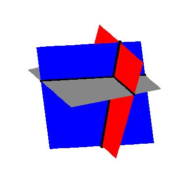
Since the geometry for equations involving more than two variables is complicated, we will focus our efforts on the algebra. Returning to the system

${\begin{matrix} x - \frac{1}{3} y + \frac{1}{2} z & = & 1 \\ y - \frac{1}{2} z & = & 4 \\ z & = & - 1 \end{matrix}$

we note the reason it was so easy to solve is that the third equation is solved for $z$ , the second equation involves only $y$ and $z$ , and since the coefficient of $y$ is $1$ , it makes it easy to solve for $y$ using our known value for $z$ . Lastly, the coefficient of $x$ in the first equation is $1$ making it easy to substitute the known values of $y$ and $z$ and then solve for $x$ . We formalize this pattern below for the most general systems of linear equations. Again, we use subscripted variables to describe the general case. The variable with the smallest subscript in a given equation is typically called the leading variable of that equation.

In our previous system, if we make the obvious choices $x equals x sub 1$ , $y equals x sub 2$ , and $z equals x sub 3$ , we see that the system is in triangular form.¹⁴ An example of a more complicated system in triangular form is

${\begin{matrix} x_{1} - 4 x_{3} + x_{4} - x_{6} & = & 6 \\ x_{2} + 2 x_{3} & = & 1 \\ x_{4} + 3 x_{5} - x_{6} & = & 8 \\ x_{5} + 9 x_{6} & = & 10 \end{matrix}$

Our goal henceforth will be to transform a given system of linear equations into triangular form using the moves in Theorem.

Example 2

Use Theorem to put the following systems into triangular form and then solve the system if possible. Classify each system as consistent independent, consistent dependent, or inconsistent.

${\begin{matrix} 3 x - y + z & = & 3 \\ 2 x - 4 y + 3 z & = & 16 \\ x - y + z & = & 5 \end{matrix}$
${\begin{matrix} 2 x + 3 y - z & = & 1 \\ 10 x - z & = & 2 \\ 4 x - 9 y + 2 z & = & 5 \end{matrix}$
${\begin{matrix} 3 x_{1} + x_{2} + x_{4} & = & 6 \\ 2 x_{1} + x_{2} - x_{3} & = & 4 \\ x_{2} - 3 x_{3} - 2 x_{4} & = & 0 \end{matrix}$

For definitiveness, we label the topmost equation in the system $E ⁢ 1$ , the equation beneath that $E ⁢ 2$ , and so forth. We now attempt to put the system in triangular form using an algorithm known as Gaussian Elimination. What this means is that, starting with $x$ , we transform the system so that conditions 2 and 3 in Definition are satisfied. Then we move on to the next variable, in this case $y$ , and repeat. Since the variables in all of the equations have a consistent ordering from left to right, our first move is to get an $x$ in $E ⁢ 1$ 's spot with a coefficient of $1$ . While there are many ways to do this, the easiest is to apply the first move listed in Theorem and interchange $E ⁢ 1$ and $E ⁢ 3$ .
$\begin{matrix} {\begin{matrix} (E 1) & 3 x - y + z & = & 3 \\ (E 2) & 2 x - 4 y + 3 z & = & 16 \\ (E 3) & x - y + z & = & 5 \end{matrix} & \overset{Switch E 1 and E 3}{\to} & {\begin{matrix} (E 1) & x - y + z & = & 5 \\ (E 2) & 2 x - 4 y + 3 z & = & 16 \\ (E 3) & 3 x - y + z & = & 3 \end{matrix} \end{matrix}$
To satisfy Definition, we need to eliminate the $x$ 's from $E ⁢ 2$ and $E ⁢ 3$ . We accomplish this by replacing each of them with a sum of themselves and a multiple of $E ⁢ 1$ . To eliminate the $x$ from $E ⁢ 2$ , we need to multiply $E ⁢ 1$ by $minus 2$ then add; to eliminate the $x$ from $E ⁢ 3$ , we need to multiply $E ⁢ 1$ by $minus 3$ then add. Applying the third move listed in Theorem twice, we get
$\begin{matrix} {\begin{matrix} (E 1) & x - y + z & = & 5 \\ (E 2) & 2 x - 4 y + 3 z & = & 16 \\ (E 3) & 3 x - y + z & = & 3 \end{matrix} & \to_{Replace E 3 with ¯ 3 E 1 + E 3}^{Replace E 2 with ¯ 2 E 1 + E 2} & {\begin{matrix} (E 1) & x - y + z & = & 5 \\ (E 2) & - 2 y + z & = & 6 \\ (E 3) & 2 y - 2 z & = & - 12 \end{matrix} \end{matrix}$
Now we enforce the conditions stated in Definition for the variable $y$ . To that end we need to get the coefficient of $y$ in $E ⁢ 2$ equal to $1$ . We apply the second move listed in Theorem and replace $E ⁢ 2$ with itself times $- \frac{1}{2}$ .
$\begin{matrix} {\begin{matrix} (E 1) & x - y + z & = & 5 \\ (E 2) & - 2 y + z & = & 6 \\ (E 3) & 2 y - 2 z & = & - 12 \end{matrix} & \overset{Replace E 2 with ¯ \frac{1}{2} E 2}{\to} & {\begin{matrix} (E 1) & x - y + z & = & 5 \\ (E 2) & y - \frac{1}{2} z & = & - 3 \\ (E 3) & 2 y - 2 z & = & - 12 \end{matrix} \end{matrix}$
To eliminate the $y$ in $E ⁢ 3$ , we add $minus 2 ⁢ E ⁢ 2$ to it.
$\begin{matrix} {\begin{matrix} (E 1) & x - y + z & = & 5 \\ (E 2) & y - \frac{1}{2} z & = & - 3 \\ (E 3) & 2 y - 2 z & = & - 12 \end{matrix} & \overset{Replace E 3 with ¯ 2 E 2 + E 3}{\to} & {\begin{matrix} (E 1) & x - y + z & = & 5 \\ (E 2) & y - \frac{1}{2} z & = & - 3 \\ (E 3) & - z & = & - 6 \end{matrix} \end{matrix}$
Finally, we apply the second move from Theorem one last time and multiply $E ⁢ 3$ by $minus 1$ to satisfy the conditions of Definition for the variable $z$ .
$\begin{matrix} {\begin{matrix} (E 1) & x - y + z & = & 5 \\ (E 2) & y - \frac{1}{2} z & = & - 3 \\ (E 3) & - z & = & - 6 \end{matrix} & \overset{Replace E 3 with ¯ 1 E 3}{\to} & {\begin{matrix} (E 1) & x - y + z & = & 5 \\ (E 2) & y - \frac{1}{2} z & = & - 3 \\ (E 3) & z & = & 6 \end{matrix} \end{matrix}$
Now we proceed to substitute. Plugging in $z equals 6$ into $E ⁢ 2$ gives $y - 3 = - 3$ so that $y equals 0$ . With $y equals 0$ and $z equals 6$ , $E ⁢ 1$ becomes $x - 0 + 6 = 5$ , or $x = - 1$ . Our solution is $open parenthesis minus 1, 0, 6 close parenthesis$ . We leave it to the reader to check that substituting the respective values for $x$ , $y$ , and $z$ into the original system results in three identities. Since we have found a solution, the system is consistent; since there are no free variables, it is independent.
Proceeding as we did in 1, our first step is to get an equation with $x$ in the $E ⁢ 1$ position with $1$ as its coefficient. Since there is no easy fix, we multiply $E ⁢ 1$ by $\frac{1}{2}$ .
$\begin{matrix} {\begin{matrix} (E 1) & 2 x + 3 y - z & = & 1 \\ (E 2) & 10 x - z & = & 2 \\ (E 3) & 4 x - 9 y + 2 z & = & 5 \end{matrix} & \overset{Replace E 1 with \frac{1}{2} E 1}{\to} & {\begin{matrix} (E 1) & x + \frac{3}{2} y - \frac{1}{2} z & = & \frac{1}{2} \\ (E 2) & 10 x - z & = & 2 \\ (E 3) & 4 x - 9 y + 2 z & = & 5 \end{matrix} \end{matrix}$
Now it's time to take care of the $x$ 's in $E ⁢ 2$ and $E ⁢ 3$ .
$\begin{matrix} {\begin{matrix} (E 1) & x + \frac{3}{2} y - \frac{1}{2} z & = & \frac{1}{2} \\ (E 2) & 10 x - z & = & 2 \\ (E 3) & 4 x - 9 y + 2 z & = & 5 \end{matrix} & \to_{Replace E 3 with ¯ 4 E 1 + E 3}^{Replace E 2 with ¯ 10 E 1 + E 2} & {\begin{matrix} (E 1) & x + \frac{3}{2} y - \frac{1}{2} z & = & \frac{1}{2} \\ (E 2) & - 15 y + 4 z & = & - 3 \\ (E 3) & - 15 y + 4 z & = & 3 \end{matrix} \end{matrix}$
Our next step is to get the coefficient of $y$ in $E ⁢ 2$ equal to $1$ . To that end, we have
$\begin{matrix} {\begin{matrix} (E 1) & x + \frac{3}{2} y - \frac{1}{2} z & = & \frac{1}{2} \\ (E 2) & - 15 y + 4 z & = & - 3 \\ (E 3) & - 15 y + 4 z & = & 3 \end{matrix} & \overset{Replace E 2 with ¯ \frac{1}{15} E 2}{\to} & {\begin{matrix} (E 1) & x + \frac{3}{2} y - \frac{1}{2} z & = & \frac{1}{2} \\ (E 2) & y - \frac{4}{15} z & = & \frac{1}{5} \\ (E 3) & - 15 y + 4 z & = & 3 \end{matrix} \end{matrix}$
Finally, we rid $E ⁢ 3$ of $y$ .
$\begin{matrix} {\begin{matrix} (E 1) & x + \frac{3}{2} y - \frac{1}{2} z & = & \frac{1}{2} \\ (E 2) & y - \frac{4}{15} z & = & \frac{1}{5} \\ (E 3) & - 15 y + 4 z & = & 3 \end{matrix} & \overset{Replace E 3 with 15 E 2 + E 3}{\to} & {\begin{matrix} (E 1) & x - y + z & = & 5 \\ (E 2) & y - \frac{1}{2} z & = & - 3 \\ (E 3) & 0 & = & 6 \end{matrix} \end{matrix}$
The last equation, $0 equals 6$ , is a contradiction so the system has no solution. According to Theorem, since this system has no solutions, neither does the original, thus we have an inconsistent system.
For our last system, we begin by multiplying $E ⁢ 1$ by $\frac{1}{3}$ to get a coefficient of $1$ on $x sub 1$ .
$\begin{matrix} {\begin{matrix} (E 1) & 3 x_{1} + x_{2} + x_{4} & = & 6 \\ (E 2) & 2 x_{1} + x_{2} - x_{3} & = & 4 \\ (E 3) & x_{2} - 3 x_{3} - 2 x_{4} & = & 0 \end{matrix} & \overset{Replace E 1 with \frac{1}{3} E 1}{\to} & {\begin{matrix} (E 1) & x_{1} + \frac{1}{3} x_{2} + \frac{1}{3} x_{4} & = & 2 \\ (E 2) & 2 x_{1} + x_{2} - x_{3} & = & 4 \\ (E 3) & x_{2} - 3 x_{3} - 2 x_{4} & = & 0 \end{matrix} \end{matrix}$
Next we eliminate $x sub 1$ from $E ⁢ 2$
$\begin{matrix} {\begin{matrix} (E 1) & x_{1} + \frac{1}{3} x_{2} + \frac{1}{3} x_{4} & = & 2 \\ (E 2) & 2 x_{1} + x_{2} - x_{3} & = & 4 \\ (E 3) & x_{2} - 3 x_{3} - 2 x_{4} & = & 0 \end{matrix} & \to_{with ¯ 2 E 1 + E 2}^{Replace E 2} & {\begin{matrix} (E 1) & x_{1} + \frac{1}{3} x_{2} + \frac{1}{3} x_{4} & = & 2 \\ (E 2) & \frac{1}{3} x_{2} - x_{3} - \frac{2}{3} x_{4} & = & 0 \\ (E 3) & x_{2} - 3 x_{3} - 2 x_{4} & = & 0 \end{matrix} \end{matrix}$
We switch $E ⁢ 2$ and $E ⁢ 3$ to get a coefficient of $1$ for $x sub 2$ .
$\begin{matrix} {\begin{matrix} (E 1) & x_{1} + \frac{1}{3} x_{2} + \frac{1}{3} x_{4} & = & 2 \\ (E 2) & \frac{1}{3} x_{2} - x_{3} - \frac{2}{3} x_{4} & = & 0 \\ (E 3) & x_{2} - 3 x_{3} - 2 x_{4} & = & 0 \end{matrix} & \overset{Switch E 2 and E 3}{\to} & {\begin{matrix} (E 1) & x_{1} + \frac{1}{3} x_{2} + \frac{1}{3} x_{4} & = & 2 \\ (E 2) & x_{2} - 3 x_{3} - 2 x_{4} & = & 0 \\ (E 3) & \frac{1}{3} x_{2} - x_{3} - \frac{2}{3} x_{4} & = & 0 \end{matrix} \end{matrix}$
Finally, we eliminate $x sub 2$ in $E ⁢ 3$ .
$\begin{matrix} {\begin{matrix} (E 1) & x_{1} + \frac{1}{3} x_{2} + \frac{1}{3} x_{4} & = & 2 \\ (E 2) & x_{2} - 3 x_{3} - 2 x_{4} & = & 0 \\ (E 3) & \frac{1}{3} x_{2} - x_{3} - \frac{2}{3} x_{4} & = & 0 \end{matrix} & \to_{with ¯ \frac{1}{3} E 2 + E 3}^{Replace E 3} & {\begin{matrix} (E 1) & x_{1} + \frac{1}{3} x_{2} + \frac{1}{3} x_{4} & = & 2 \\ (E 2) & x_{2} - 3 x_{3} - 2 x_{4} & = & 0 \\ (E 3) & 0 & = & 0 \end{matrix} \end{matrix}$
Equation $E ⁢ 3$ reduces to $0 equals 0$ ,which is always true. Since we have no equations with $x sub 3$ or $x sub 4$ as leading variables, they are both free, which means we have a consistent dependent system. We parametrize the solution set by letting $x sub 3 equals s$ and $x sub 4 equals t$ and obtain from $E ⁢ 2$ that $x_{2} = 3 s + 2 t$ . Substituting this and $x sub 4 equals t$ into $E ⁢ 1$ , we have $x_{1} + \frac{1}{3} (3 s + 2 t) + \frac{1}{3} t = 2$ which gives $x_{1} = 2 - s - t$ . Our solution is the set ${(2 - s - t, 2 s + 3 t, s, t) | - \infty < s, t < \infty}$ .¹⁵ We leave it to the reader to verify that the substitutions $x_{1} = 2 - s - t$ , $x_{2} = 3 s + 2 t$ , $x sub 3 equals s$ and $x sub 4 equals t$ satisfy the equations in the original system.

Like all algorithms, Gaussian Elimination has the advantage of always producing what we need, but it can also be inefficient at times. For example, when solving 2 above, it is clear after we eliminated the $x$ 's in the second step to get the system

${\begin{matrix} (E 1) & x + \frac{3}{2} y - \frac{1}{2} z & = & \frac{1}{2} \\ (E 2) & - 15 y + 4 z & = & - 3 \\ (E 3) & - 15 y + 4 z & = & 3 \end{matrix}$

that equations $E ⁢ 2$ and $E ⁢ 3$ when taken together form a contradiction since we have identical left hand sides and different right hand sides. The algorithm takes two more steps to reach this contradiction. We also note that substitution in Gaussian Elimination is delayed until all the elimination is done, thus it gets called back-substitution. This may also be inefficient in many cases. Rest assured, the technique of substitution as you may have learned it in Intermediate Algebra will once again take center stage in Section. Lastly, we note that the system in 3 above is underdetermined, and as it is consistent, we have free variables in our answer. We close this section with a standard `mixture' type application of systems of linear equations.

Example 3

Lucas needs to create a $500$ milliliters (mL) of a $40 %$ acid solution. He has stock solutions of $30 %$ and $90 %$ acid as well as all of the distilled water he wants. Set-up and solve a system of linear equations which determines all of the possible combinations of the stock solutions and water which would produce the required solution.

We are after three unknowns, the amount (in mL) of the $30 %$ stock solution (which we'll call $x$ ), the amount (in mL) of the $90 %$ stock solution (which we'll call $y$ ) and the amount (in mL) of water (which we'll call $w$ ). We now need to determine some relationships between these variables. Our goal is to produce $500$ milliliters of a $40 %$ acid solution. This product has two defining characteristics. First, it must be $500$ mL; second, it must be $40 %$ acid. We take each of these qualities in turn. First, the total volume of $500$ mL must be the sum of the contributed volumes of the two stock solutions and the water. That is

$amount of 30 % stock solution + amount of 90 % stock solution + amount of water = 500 mL$

Using our defined variables, this reduces to $x + y + w = 500$ . Next, we need to make sure the final solution is $40 %$ acid. Since water contains no acid, the acid will come from the stock solutions only. We find $40 %$ of $500$ mL to be $200$ mL which means the final solution must contain $200$ mL of acid. We have

$amount of acid in 30 % stock solution + amount of acid 90 % stock solution = 200 mL$

The amount of acid in $x$ mL of $30 %$ stock is $0.30 ⁢ x$ and the amount of acid in $y$ mL of $90 %$ solution is $0.90 ⁢ y$ . We have $0.30 x + 0.90 y = 200$ . Converting to fractions,¹⁶ our system of equations becomes

${\begin{matrix} x + y + w & = & 500 \\ \frac{3}{10} x + \frac{9}{10} y & = & 200 \end{matrix}$

We first eliminate the $x$ from the second equation

$\begin{matrix} {\begin{matrix} (E 1) & x + y + w & = & 500 \\ (E 2) & \frac{3}{10} x + \frac{9}{10} y & = & 200 \end{matrix} & \overset{Replace E 2 with ¯ \frac{3}{10} E 1 + E 2}{\to} & {\begin{matrix} (E 1) & x + y + w & = & 500 \\ (E 2) & \frac{3}{5} y - \frac{3}{10} w & = & 50 \end{matrix} \end{matrix}$

Next, we get a coefficient of $1$ on the leading variable in $E ⁢ 2$

$\begin{matrix} {\begin{matrix} (E 1) & x + y + w & = & 500 \\ (E 2) & \frac{3}{5} y - \frac{3}{10} w & = & 50 \end{matrix} & \overset{Replace E 2 with \frac{5}{3} E 2}{\to} & {\begin{matrix} (E 1) & x + y + w & = & 500 \\ (E 2) & y - \frac{1}{2} w & = & \frac{250}{3} \end{matrix} \end{matrix}$

Notice that we have no equation to determine $w$ , and as such, $w$ is free. We set $w = t$ and from $E ⁢ 2$ get $y = \frac{1}{2} t + \frac{250}{3}$ . Substituting into $E ⁢ 1$ gives $x + (\frac{1}{2} t + \frac{250}{3}) + t = 500$ so that $x = - \frac{3}{2} t + \frac{1250}{3}$ . This system is consistent, dependent and its solution set is ${(- \frac{3}{2} t + \frac{1250}{3}, \frac{1}{2} t + \frac{250}{3}, t) | - \infty < t < \infty}$ . While this answer checks algebraically, we have neglected to take into account that $x$ , $y$ and $w$ , being amounts of acid and water, need to be nonnegative. That is, $x greater than or equal to 0$ , $y greater than or equal to 0$ and $w greater than or equal to 0$ . The constraint $x greater than or equal to 0$ gives us $- \frac{3}{2} t + \frac{1250}{3} \geq 0$ , or $t \leq \frac{2500}{9}$ . From $y greater than or equal to 0$ , we get $\frac{1}{2} t + \frac{250}{3} \geq 0$ or $t \geq - \frac{500}{3}$ . The condition $z greater than or equal to 0$ yields $t greater than or equal to 0$ , and we see that when we take the set theoretic intersection of these intervals, we get $0 \leq t \leq \frac{2500}{9}$ . Our final answer is ${(- \frac{3}{2} t + \frac{1250}{3}, \frac{1}{2} t + \frac{250}{3}, t) | 0 \leq t \leq \frac{2500}{9}}$ . Of what practical use is our answer? Suppose there is only $100$ mL of the $90 %$ solution remaining and it is due to expire. Can we use all of it to make our required solution? We would have $y equals 100$ so that $\frac{1}{2} t + \frac{250}{3} = 100$ , and we get $t = \frac{100}{3}$ . This means the amount of $30 %$ solution required is $x = - \frac{3}{2} t + \frac{1250}{3} = - \frac{3}{2} (\frac{100}{3}) + \frac{1250}{3} = \frac{1100}{3}$ mL, and for the water, $w = t = \frac{100}{3}$ mL. The reader is invited to check that mixing these three amounts of our constituent solutions produces the required $40 %$ acid mix.

Exercises

(Review Exercises) In Exercises -, take a trip down memory lane and solve the given system using substitution and/or elimination. Classify each system as consistent independent, consistent dependent, or inconsistent. Check your answers both algebraically and graphically.

${\begin{matrix} x + 2 y & = & 5 \\ x & = & 6 \end{matrix}$
${\begin{matrix} 2 y - 3 x & = & 1 \\ y & = & - 3 \end{matrix}$
${\begin{matrix} \frac{x + 2 y}{4} & = & - 5 \\ \frac{3 x - y}{2} & = & 1 \end{matrix}$
${\begin{matrix} \frac{2}{3} x - \frac{1}{5} y & = & 3 \\ \frac{1}{2} x + \frac{3}{4} y & = & 1 \end{matrix}$
${\begin{matrix} \frac{1}{2} x - \frac{1}{3} y & = & - 1 \\ 2 y - 3 x & = & 6 \end{matrix}$
${\begin{matrix} x + 4 y & = & 6 \\ \frac{1}{12} x + \frac{1}{3} y & = & \frac{1}{2} \end{matrix}$
${\begin{matrix} 3 y - \frac{3}{2} x & = & - \frac{15}{2} \\ \frac{1}{2} x - y & = & \frac{3}{2} \end{matrix}$
${\begin{matrix} \frac{5}{6} x + \frac{5}{3} y & = & - \frac{7}{3} \\ - \frac{10}{3} x - \frac{20}{3} y & = & 10 \end{matrix}$
${\begin{matrix} - 5 x + y & = & 17 \\ x + y & = & 5 \end{matrix}$
${\begin{matrix} x + y + z & = & 3 \\ 2 x - y + z & = & 0 \\ - 3 x + 5 y + 7 z & = & 7 \end{matrix}$
${\begin{matrix} 4 x - y + z & = & 5 \\ 2 y + 6 z & = & 30 \\ x + z & = & 5 \end{matrix}$
${\begin{matrix} 4 x - y + z & = & 5 \\ 2 y + 6 z & = & 30 \\ x + z & = & 6 \end{matrix}$
${\begin{matrix} x + y + z & = & - 17 \\ y - 3 z & = & 0 \end{matrix}$
${\begin{matrix} x - 2 y + 3 z & = & 7 \\ - 3 x + y + 2 z & = & - 5 \\ 2 x + 2 y + z & = & 3 \end{matrix}$
${\begin{matrix} 3 x - 2 y + z & = & - 5 \\ x + 3 y - z & = & 12 \\ x + y + 2 z & = & 0 \end{matrix}$
${\begin{matrix} 2 x - y + z & = & - 1 \\ 4 x + 3 y + 5 z & = & 1 \\ 5 y + 3 z & = & 4 \end{matrix}$
${\begin{matrix} x - y + z & = & - 4 \\ - 3 x + 2 y + 4 z & = & - 5 \\ x - 5 y + 2 z & = & - 18 \end{matrix}$
${\begin{matrix} 2 x - 4 y + z & = & - 7 \\ x - 2 y + 2 z & = & - 2 \\ - x + 4 y - 2 z & = & 3 \end{matrix}$
${\begin{matrix} 2 x - y + z & = & 1 \\ 2 x + 2 y - z & = & 1 \\ 3 x + 6 y + 4 z & = & 9 \end{matrix}$
${\begin{matrix} x - 3 y - 4 z & = & 3 \\ 3 x + 4 y - z & = & 13 \\ 2 x - 19 y - 19 z & = & 2 \end{matrix}$
${\begin{matrix} x + y + z & = & 4 \\ 2 x - 4 y - z & = & - 1 \\ x - y & = & 2 \end{matrix}$
${\begin{matrix} x - y + z & = & 8 \\ 3 x + 3 y - 9 z & = & - 6 \\ 7 x - 2 y + 5 z & = & 39 \end{matrix}$
${\begin{matrix} 2 x - 3 y + z & = & - 1 \\ 4 x - 4 y + 4 z & = & - 13 \\ 6 x - 5 y + 7 z & = & - 25 \end{matrix}$
${\begin{matrix} 2 x_{1} + x_{2} - 12 x_{3} - x_{4} & = & 16 \\ - x_{1} + x_{2} + 12 x_{3} - 4 x_{4} & = & - 5 \\ 3 x_{1} + 2 x_{2} - 16 x_{3} - 3 x_{4} & = & 25 \\ x_{1} + 2 x_{2} - 5 x_{4} & = & 11 \end{matrix}$
${\begin{matrix} x_{1} - x_{3} & = & - 2 \\ 2 x_{2} - x_{4} & = & 0 \\ x_{1} - 2 x_{2} + x_{3} & = & 0 \\ - x_{3} + x_{4} & = & 1 \end{matrix}$
${\begin{matrix} x_{1} - x_{2} - 5 x_{3} + 3 x_{4} & = & - 1 \\ x_{1} + x_{2} + 5 x_{3} - 3 x_{4} & = & 0 \\ x_{2} + 5 x_{3} - 3 x_{4} & = & 1 \\ x_{1} - 2 x_{2} - 10 x_{3} + 6 x_{4} & = & - 1 \end{matrix}$
Find two other forms of the parametric solution to Exercise above by reorganizing the equations so that $x$ or $y$ can be the free variable.
A local buffet charges $$ 7.50$ per person for the basic buffet and $$ 9.25$ for the deluxe buffet (which includes crab legs.) If 27 diners went out to eat and the total bill was $$ 227.00$ before taxes, how many chose the basic buffet and how many chose the deluxe buffet?
At The Old Home Fill'er Up and Keep on a-Truckin' Cafe, Mavis mixes two different types of coffee beans to produce a house blend. The first type costs $3 per pound and the second costs $8 per pound. How much of each type does Mavis use to make 50 pounds of a blend which costs $6 per pound?
Skippy has a total of $$$ 10,000 to split between two investments. One account offers $3 %$ simple interest, and the other account offers $8 %$ simple interest. For tax reasons, he can only earn $$ 500$ in interest the entire year. How much money should Skippy invest in each account to earn $$ 500$ in interest for the year?
A $10 %$ salt solution is to be mixed with pure water to produce 75 gallons of a $3 %$ salt solution. How much of each are needed?
At The Crispy Critter's Head Shop and Patchouli Emporium along with their dried up weeds, sunflower seeds and astrological postcards they sell an herbal tea blend. By weight, Type I herbal tea is 30% peppermint, 40% rose hips and 30% chamomile, Type II has percents 40%, 20% and 40%, respectively, and Type III has percents 35%, 30% and 35%, respectively. How much of each Type of tea is needed to make 2 pounds of a new blend of tea that is equal parts peppermint, rose hips and chamomile?
Discuss with your classmates how you would approach Exercise above if they needed to use up a pound of Type I tea to make room on the shelf for a new canister.
If you were to try to make 100 mL of a $60 %$ acid solution using stock solutions at $20 %$ and $40 %$ , respectively, what would the triangular form of the resulting system look like? Explain.

In Exercises -, put each system of linear equations into triangular form and solve the system if possible. Classify each system as consistent independent, consistent dependent, or inconsistent.

Answers

Consistent independent Solution $(6, - \frac{1}{2})$
Consistent independent Solution $(- \frac{7}{3}, - 3)$
Consistent independent Solution $(- \frac{16}{7}, - \frac{62}{7})$
Consistent independent Solution $(\frac{49}{12}, - \frac{25}{18})$
Consistent dependent Solution $(t, \frac{3}{2} t + 3)$ for all real numbers $t$
Consistent dependent Solution $open parenthesis 6 minus 4 ⁢ t, t close parenthesis$ for all real numbers $t$
Inconsistent No solution
Inconsistent No solution
If $x$ is the free variable then the solution is $(t, 3 t, - t + 5)$ and if $y$ is the free variable then the solution is $(\frac{1}{3} t, t, - \frac{1}{3} t + 5)$ .
$13$ chose the basic buffet and $14$ chose the deluxe buffet.
Mavis needs 20 pounds of $3 per pound coffee and 30 pounds of $8 per pound coffee.
Skippy needs to invest $$$ 6000 in the $3 %$ account and $$$ 4000 in the $8 %$ account.
$22.5$ gallons of the $10 %$ solution and $52.5$ gallons of pure water.
$\frac{4}{3} - \frac{1}{2} t$ pounds of Type I, $\frac{2}{3} - \frac{1}{2} t$ pounds of Type II and $t$ pounds of Type III where $0 \leq t \leq \frac{4}{3}$ .

Because triangular form is not unique, we give only one possible answer to that part of the question. Yours may be different and still be correct.

Critics may argue that $x equals 5$ is clearly an equation in one variable. It can also be considered an equation in $117$ variables with the coefficients of $116$ variables set to $0$ . As with many conventions in Mathematics, the context will clarify the situation. ↩
See Section for a review of this. ↩
Note that we could have just as easily chosen to solve $2 x - 4 y = 6$ for $x$ to obtain $x = 2 y + 3$ . Letting $y$ be the parameter $t$ , we have that for any value of $t$ , $x = 2 t + 3$ , which gives ${(2 t + 3, t) | - \infty < t < \infty}$ . There is no one correct way to parameterize the solution set, which is why it is always best to check your answer. ↩
In the case of systems of linear equations, regardless of the number of equations or variables, consistent independent systems have exactly one solution. The reader is encouraged to think about why this is the case for linear equations in two variables. Hint: think geometrically. ↩
The adjectives `dependent' and `independent' apply only to consistent systems – they describe the type of solutions. Is there a free variable (dependent) or not (independent)? ↩
If we think if each variable being an unknown quantity, then ostensibly, to recover two unknown quantities, we need two pieces of information - i.e., two equations. Having more than two equations suggests we have more information than necessary to determine the values of the unknowns. While this is not necessarily the case, it does explain the choice of terminology `overdetermined'. ↩
We need more than two variables to give an example of the latter. ↩
Again, experience with systems with more variables helps to see this here, as does a solid course in Linear Algebra. ↩
That is, a system with the same solution set. ↩
That is, an equation which results from multiplying both sides of the equation by the same nonzero number. ↩
You were asked to think about this in Exercise in Section . ↩
In fact, these lines are described by the parametric solutions to the systems formed by taking any two of these equations by themselves. ↩
necessarily an identity or contradiction ↩
If letters are used instead of subscripted variables, Definition can be suitably modified using alphabetical order of the variables instead of numerical order on the subscripts of the variables. ↩
Here, any choice of $s$ and $t$ will determine a solution which is a point in $4$ -dimensional space. Yeah, we have trouble visualizing that, too. ↩
We do this only because we believe students can use all of the practice with fractions they can get! ↩

Adapted from Precalculus, 3rd corrected edition, by Carl Stitz and Jeff Zeager (stitz-zeager.com), licensed under CC BY-NC-SA 3.0. Changes were made: reformatted as an accessible XYZ web edition. License: CC-BY-NC-SA-3.0.