6.2 Graphs of the Normal Distribution

Many real life problems produce a histogram that is a symmetric, unimodal, and bell-shaped continuous probability distribution. For example: height, blood pressure, and cholesterol level. However, not every bell shaped curve is a normal curve. In a normal curve, there is a specific relationship between its “height” and its “width.”

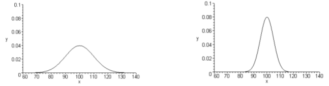
Normal curves can be tall and skinny or they can be short and fat. They are all symmetric, unimodal, and centered at $\mu$, the population mean. Figure $1$ shows two different normal curves drawn on the same scale. Both have $\mu =100$ but the one on the left has a standard deviation of 10 and the one on the right has a standard deviation of 5. Notice that the larger standard deviation makes the graph wider (more spread out) and shorter.

Every normal curve has common features. These are detailed in Figure $2$.

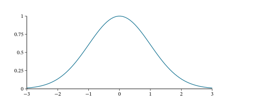
• The center, or the highest point, is at the population mean, $\mu$.
• The transition points (inflection points) are the places where the curve changes from a “hill” to a “valley”. The distance from the mean to the transition point is one standard deviation, $\sigma$.
• The area under the whole curve is exactly 1. Therefore, the area under the half below or above the mean is 0.5.

The equation that creates this curve is $f(x)=\frac{1}{\sigma \sqrt{2\pi }}{e}^{-\frac{1}{2}{\left(\frac{x-\mu }{\sigma }\right)}^2}$

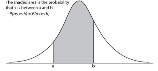
Just as in a discrete probability distribution, the object is to find the probability of an event occurring. However, unlike in a discrete probability distribution where the event can be a single value, in a continuous probability distribution the event must be a range. You are interested in finding the probability of x occurring in the range between a and b, or $$P(a\le x\le b)=P(a<x<b)$$. Calculus tells us that to find this you find the area under the curve above the interval from a to b.

$$P(a\le x\le b)=P(a<x<b)$$ is the area under the curve above the interval from a to b.

Before looking at the process for finding the probabilities under the normal curve, it is somewhat useful to look at the Empirical Rule that gives approximate values for these areas. The Empirical Rule is just an approximation and it will only be used in this section to give you an idea of what the size of the probabilities is for different shadings. A more precise method for finding probabilities for the normal curve will be demonstrated in the next section. Please do not use the empirical rule except for real rough estimates.

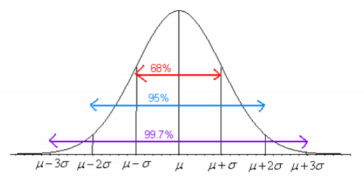
Be careful, there is still some area left over in each end. Remember, the maximum a probability can be is 100%, so if you calculate 100%-99.7%=0.3% you will see that for both ends together there is 0.3% of the curve. Because of symmetry, you can divide this equally between both ends and find that there is 0.15% in each tail beyond the $\mu \pm 3\sigma$.