3.2 Measures of Spread

Variability is an important idea in statistics. If you were to measure the height of everyone in your classroom, every observation gives you a different value. That means not every student has the same height. Thus there is variability in people’s heights. If you were to take a sample of the income level of people in a town, every sample gives you different information. There is variability between samples too. Variability describes how the data are spread out. If the data are very close to each other, then there is low variability. If the data are very spread out, then there is high variability. How do you measure variability? It would be good to have a number that measures it. This section will describe some of the different measures of variability, also known as variation.

In Example $1$ , the average weight of a cat was calculated to be 8.02 pounds. How much does this tell you about the weight of all cats? Can you tell if most of the weights were close to 8.02 or were the weights really spread out? What are the highest weight and the lowest weight? All you know is that the center of the weights is 8.02 pounds. You need more information.

Example 1 Finding the Range

Look at the following three sets of data. Find the range of each of these.

$10, 20, 30, 40, 50$
$10, 29, 30, 31, 50$
$28, 29, 30, 31, 32$

Show solution

Figure

1

: Dot Plot for Example

1

Figure

2

: Dot Plot for Example

1

Figure

3

: Dot Plot for Example

1

Based on the mean, median, and range in Example $1$ , the first two distributions are the same, but you can see from the graphs that they are different. In Example $1$ a the data are spread out equally. In Example $1$ b the data has a clump in the middle and a single value at each end. The mean and median are the same for Example $1$ c but the range is very different. All the data is clumped together in the middle.

The range doesn’t really provide a very accurate picture of the variability. A better way to describe how the data is spread out is needed. Instead of looking at the distance the highest value is from the lowest how about looking at the distance each value is from the mean. This distance is called the deviation.

Example 2 Finding the Deviations

Suppose a vet wants to analyze the weights of cats. The weights (in pounds) of five cats are 6.8, 8.2, 7.5, 9.4, and 8.2. Find the deviation for each of the data values.

Show solution

Variable: $x =$ weight of a cat

The mean for this data set is $x ― equals 8.02$ pounds.

Table $1$ : Deviations of Weights of Cats
$x$	$x - \overset{―}{x}$
6.8	6.8-8.02 = -1.22
8.2	8.2-8.02=0.18
7.5	7.5-8.02=-0.52
9.4	9.4-8.02=1.38
8.2	8.2-8.02=0.18

Now you might want to average the deviation, so you need to add the deviations together.

Table $2$ : Sum of Deviations of Weights of Cats
$x$	$x - \overset{―}{x}$
6.8	6.8-8.02 = -1.22
8.2	8.2-8.02=0.18
7.5	7.5-8.02=-0.52
9.4	9.4-8.02=1.38
8.2	8.2-8.02=0.18
Total	0

This can’t be right. The average distance from the mean cannot be 0. The reason it adds to 0 is because there are some positive and negative values. You need to get rid of the negative signs. How can you do that? You could square each deviation.

Table $3$ : Squared Deviations of Weights of Cats
$x$	$x - \overset{―}{x}$	$(x - \overset{―}{x})^{2}$
6.8	6.8-8.02 = -1.22	1.4884
8.2	8.2-8.02=0.18	0.0324
7.5	7.5-8.02=-0.52	0.2704
9.4	9.4-8.02=1.38	1.9044
8.2	8.2-8.02=0.18	0.0324
Total	0	3.728

Now average the total of the squared deviations. The only thing is that in statistics there is a strange average here. Instead of dividing by the number of data values you divide by the number of data values minus 1. In this case you would have

$s^{2} = \frac{3.728}{5 - 1} = \frac{3.728}{4} = 0.932 {pounds}^{2}$

Notice that this is denoted as $s^{2}$ . This is called the variance and it is a measure of the average squared distance from the mean. If you now take the square root, you will get the average distance from the mean. This is called the standard deviation, and is denoted with the letter $s$ .

$s = \sqrt{.932} \approx 0.965$ pounds

The standard deviation is the average (mean) distance from a data point to the mean. It can be thought of as how much a typical data point differs from the mean.

Definition

Sample Variance

The sample variance formula:

$s^{2} = \frac{\sum (x - \overset{―}{x})^{2}}{n - 1}$

where $\overset{―}{x}$ is the sample mean, $n$ is the sample size, and $∑$ means to find the sum.

Definition

Sample Standard Deviation

The sample standard deviation formula:

$s = \sqrt{s^{2}} = \sqrt{\frac{\sum (x - \overset{―}{x})^{2}}{n - 1}}$

The $n minus 1$ on the bottom has to do with a concept called degrees of freedom. Basically, it makes the sample standard deviation a better approximation of the population standard deviation.

Definition

Population Standard Deviation

The population standard deviation formula:

$σ = \sqrt{σ^{2}} = \sqrt{\frac{\sum (x - μ)^{2}}{N}}$

Example 3 Finding the Standard Deviation

Suppose that a manager wants to test two new training programs. He randomly selects 5 people for each training type and measures the time it takes to complete a task after the training. The times for both trainings are in Example $4$ . Which training method is better?

Table $4$ : Time to Finish Task in Minutes
Training 1	56	75	48	63	59
Training 2	60	58	66	59	58

Show solution

It is important that you define what each variable is since there are two of them.

Variable 1: $X sub 1 equals$ productivity from training 1

Variable 2: $X sub 2 equals$ productivity from training 2

To answer which training method better, first you need some descriptive statistics. Start with the mean for each sample.

${\overset{―}{x}}_{1} = \frac{56 + 75 + 48 + 63 + 59}{5} = 60.2$ minutes

${\overset{―}{x}}_{2} = \frac{60 + 58 + 66 + 59 + 58}{5} = 60.2$ minutes

Since both means are the same values, you cannot answer the question about which is better. Now calculate the standard deviation for each sample.

Table $5$ : Squared Deviations for Training 1
$x sub 1$	$x sub 1 minus x ― sub 1$	$open parenthesis x sub 1 minus x ― sub 1 close parenthesis squared$
56	-4.2	17.64
75	14.8	219.04
48	-12.2	148.84
63	2.8	7.84
59	-1.2	1.44
Total	0	394.8

Table $6$ : Squared Deviations for Training 2
$x sub 2$	$x sub 2 minus x ― sub 2$	$open parenthesis x sub 2 minus x ― sub 2 close parenthesis squared$
60	-0.2	0.04
58	-2.2	4.84
66	5.8	33.64
59	-1.2	1.44
58	-2.2	4.84
Total	0	44.8

The variance for each sample is:

$s_{1}^{2} = \frac{394.8}{5 - 1} = 98.7 {minutes}^{2}$

$s_{2}^{2} = \frac{44.8}{5 - 1} = 11.2 {minutes}^{2}$

The standard deviations are:

$s_{1} = \sqrt{98.7} \approx 9.93$ minutes

$s_{2} = \sqrt{11.2} \approx 3.35$ minutes

From the standard deviations, the second training seemed to be the better training since the data is less spread out. This means it is more consistent. It would be better for the managers in this case to have a training program that produces more consistent results so they know what to expect for the time it takes to complete the task.

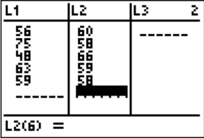
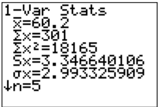
You can do the calculations for the descriptive statistics using the technology. The procedure for calculating the sample mean ( $\overset{―}{x})$ and the sample standard deviation ( $s_{x}$ ) for $X sub 2$ in Example $3$ on the TI-83/84 is in Figures 3.2.1 through 3.2.4 (the procedure is the same for $X sub 1$ ). Note the calculator gives you the population standard deviation ( $σ_{x}$ ) because it doesn’t know whether the data you input is a population or a sample. You need to decide which value you need to use, based on whether you have a population or sample. In almost all cases you have a sample and will be using $s_{x}$ . Also, the calculator uses the notation $s_{x}$ of instead of just $s$ . It is just a way for it to denote the information. First you need to go into the STAT menu, and then Edit. This will allow you to type in your data (see Figure $1$ ).

TI-84 calculator list editor screen showing values entered in L1 (56, 75, 48, 63, 59) and L2 (60, 58, 66, 59, 58), with the cursor on the sixth L2 entry. — Figure $1$ : TI-83/84 Calculator Edit Setup

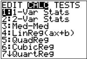
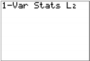
Once you have the data into the calculator, you then go back to the STAT menu, move over to CALC, and then choose 1-Var Stats (see Figure $2$ ). The calculator will now put 1-Var Stats on the main screen. Now type in L2 (2nd button and 2) and then press ENTER. (Note if you have the newer operating system on the TI-84, then the procedure is slightly different.) The results from the calculator are in Figure $4$ .

TI-83/84 calculator STAT menu with the CALC tab selected, listing 1-Var Stats, 2-Var Stats, Med-Med, LinReg(ax+b), QuadReg, CubicReg, and QuartReg (quartic regression). — Figure $2$ : TI-83/84 Calculator CALC Menu

TI-84 calculator screen displaying the command header '1-Var Stats L2' with no results yet shown. — Figure $3$ : TI-83/84 Calculator Input for Example $3$ Variable $X sub 2$

TI-84 calculator 1-Var Stats screen showing mean x̄=60.2, sums Σx=301 and Σx²=18165, sample standard deviation Sx=3.346640106, population standard deviation σx=2.993325909, and n=5. — Figure $4$ : TI-83/84 Calculator Results for Example $3$ Variable $X sub 2$

The processes for finding the mean, median, range, standard deviation, and variance on R are as follows:

variable<-c(type in your data)
To find the mean, use mean(variable)
To find the median, use median(variable)
To find the range, use range(variable). Then find maximum – minimum.
To find the standard deviation, use sd(variable)
To find the variance, use var(variable)

For the second data set in Example $3$ , the commands and results would be

productivity_2<-c(60, 58, 66, 59, 58)
mean(productivity_2)
[1] 60.2
median(productivity_2)
[1] 59
range(productivity_2)
[1] 58 66
sd(productivity_2)
[1] 3.34664
var(productivity_2)
[1] 11.2

productivity_2 <- c(60, 58, 66, 59, 58)

mean(productivity_2)

median(productivity_2)

range(productivity_2)

sd(productivity_2)

var(productivity_2)

In general a “small” standard deviation means the data is close together (more consistent) and a “large” standard deviation means the data is spread out (less consistent). Sometimes you want consistent data and sometimes you don’t. As an example if you are making bolts, you want to lengths to be very consistent so you want a small standard deviation. If you are administering a test to see who can be a pilot, you want a large standard deviation so you can tell who are the good pilots and who are the bad ones.

What do “small” and “large” mean? To a bicyclist whose average speed is 20 mph, s = 20 mph is huge. To an airplane whose average speed is 500 mph, s = 20 mph is nothing. The “size” of the variation depends on the size of the numbers in the problem and the mean. Another situation where you can determine whether a standard deviation is small or large is when you are comparing two different samples such as in example #3.2.3. A sample with a smaller standard deviation is more consistent than a sample with a larger standard deviation.

Many other books and authors stress that there is a computational formula for calculating the standard deviation. However, this formula doesn’t give you an idea of what standard deviation is and what you are doing. It is only good for doing the calculations quickly. It goes back to the days when standard deviations were calculated by hand, and the person needed a quick way to calculate the standard deviation. It is an archaic formula that this author is trying to eradicate it. It is not necessary anymore, since most calculators and computers will do the calculations for you with as much meaning as this formula gives. It is suggested that you never use it. If you want to understand what the standard deviation is doing, then you should use the definition formula. If you want an answer quickly, use a computer or calculator.

Use of Standard Deviation

One of the uses of the standard deviation is to describe how a population is distributed by using Chebyshev’s Theorem. This theorem works for any distribution, whether it is skewed, symmetric, bimodal, or any other shape. It gives you an idea of how much data is a certain distance on either side of the mean.

Example 4 Using Chebyshev's Theorem

The U.S. Weather Bureau has provided the information in Table 7 about the total annual number of reported strong to violent (F3+) tornados in the United States for the years 1954 to 2012. ("U.S. tornado climatology," 17).

Table $7$ : Annual Number of Violent Tornados in the U.S.
46	47	31	41	24	56	56	23	31	59
39	70	73	85	33	38	45	39	35	22
51	39	51	131	37	24	57	42	28	45
98	35	54	45	30	15	35	64	21	84
40	51	44	62	65	27	34	23	32	28
41	98	82	47	62	21	31	29	32

Use Chebyshev’s theorem to find an interval centered about the mean annual number of strong to violent (F3+) tornados in which you would expect at least 75% of the years to fall.
Use Chebyshev’s theorem to find an interval centered about the mean annual number of strong to violent (F3+) tornados in which you would expect at least 88.9% of the years to fall.

Show solution

a. Variable: $x =$ number of strong or violent (F3+) tornadoes Chebyshev’s theorem says that at least 75% of the data will fall in the interval from $μ minus 2 σ$ to $μ plus 2 σ$ .

You do not have the population, so you need to estimate the population mean and standard deviation using the sample mean and standard deviation. You can find the sample mean and standard deviation using technology:

$\overset{―}{x} \approx 46.24, s \approx 22.18$

So,

$μ \approx 46.24, σ \approx 22.18$

$μ - 2 σ to μ + 2 σ$

$46.24 - 2 (22.18) to 46.24 + 2 (22.18)$

$46.24 - 44.36 to 46.24 + 44.36$

$1.88 to 90.60$

Since you can’t have fractional number of tornados, round to the nearest whole number.

At least 75% of the years have between 2 and 91 strong to violent (F3+) tornados. (Actually, all but three years’ values fall in this interval, that means that $\frac{56}{59} \approx 94.9$ actually fall in the interval.)

b. Variable: $x =$ number of strong or violent (F3+) tornadoes Chebyshev’s theorem says that at least 88.9% of the data will fall in the interval from $μ minus 3 σ$ to $μ plus 3 σ$ .

$μ - 3 σ to μ + 3 σ$

$46.24 - 3 (22.18) to 46.24 + 3 (22.18)$

$46.24 - 66.54 to 46.24 + 66.54$

$minus 20.30 to 112.78$

Since you can’t have negative number of tornados, the lower limit is actually 0. Since you can’t have fractional number of tornados, round to the nearest whole number.

At least 88.9% of the years have between 0 and 113 strong to violent (F3+) tornados.

(Actually, all but one year falls in this interval, that means that $\frac{58}{59} \approx 98.3$ actually fall in the interval.)

Chebyshev’s Theorem says that at least 75% of the data is within two standard deviations of the mean. That percentage is fairly high. There isn’t much data outside two standard deviations. A rule that can be followed is that if a data value is within two standard deviations, then that value is a common data value. If the data value is outside two standard deviations of the mean, either above or below, then the number is uncommon. It could even be called unusual. An easy calculation that you can do to figure it out is to find the difference between the data point and the mean, and then divide that answer by the standard deviation. As a formula this would be

$\frac{x - μ}{σ}$ .

If you don’t know the population mean, $μ$ , and the population standard deviation, $σ$ , then use the sample mean, $\overset{―}{x}$ , and the sample standard deviation, $s$ , to estimate the population parameter values. However, realize that using the sample standard deviation may not actually be very accurate.

Example 5 determining if a value is unusual

In 1974, there were 131 strong or violent (F3+) tornados in the United States. Is this value unusual? Why or why not?
In 1987, there were 15 strong or violent (F3+) tornados in the United States. Is this value unusual? Why or why not?

Show solution

a. Variable: $x =$ number of strong or violent (F3+) tornadoes

To answer this question, first find how many standard deviations 131 is from the mean. From Example $4$ , we know $μ approximately equals 46.24$ and $σ approximately equals 22.18$ . For $x equals 131$ ,

$\frac{x - μ}{σ} = \frac{131 - 46.24}{22.18} \approx 3.82$

Since this value is more than 2, then it is unusual to have 131 strong or violent (F3+) tornados in a year.

b. Variable: $x =$ number of strong or violent (F3+) tornadoes For this question the $x equals 15$ ,

$\frac{x - μ}{σ} = \frac{15 - 46.24}{22.18} \approx - 1.41$

Since this value is between -2 and 2, then it is not unusual to have only 15 strong or violent (F3+) tornados in a year.

Homework

Your Turn

Cholesterol levels were collected from patients two days after they had a heart attack (Ryan, Joiner & Ryan, Jr, 1985) and are in Table 8. Find the mean, median, range, variance, and standard deviation using technology.
Table $8$ : Cholesterol Levels
270 236 210 142 280 272 160
220 226 242 186 266 206 318
294 282 234 224 276 282 360
310 280 278 288 288 244 236

The lengths (in kilometers) of rivers on the South Island of New Zealand that flow to the Pacific Ocean are listed in Table 9 (Lee, 1994). a. Find the mean and median.
b. Find the range.
c. Find the variance and standard deviation.

Table $9$ : Lengths of Rivers (km) Flowing to Pacific Ocean
River	Length (km)	River	Length (km)
Clarence	209	Clutha	322
Conway	48	Taieri	288
Waiau	169	Shag	72
Hurunui	138	Kakanui	64
Waipara	64	Waitaki	209
Ashley	97	Waihao	64
Waimakariri	161	Pareora	56
Selwyn	95	Rangitata	121
Rakaia	145	Ophi	80
Ashburton	90

The lengths (in kilometers) of rivers on the South Island of New Zealand that flow to the Pacific Ocean are listed in Table 9 (Lee, 1994). Table

10

: Lengths of Rivers (km) Flowing to Tasman Sea
a. Find the mean and median.
b. Find the range.
c. Find the variance and standard deviation.

River	Length (km)	River	Length (km)
Hollyford	76	Waimea	48
Cascade	64	Motueka	108
Arawhata	68	Takaka	72
Haast	64	Aorere	72
Karangarua	37	Heaphy	35
Cook	32	Karamea	80
Waiho	32	Mokihinui	56
Whataroa	51	Buller	177
Wanganui	56	Grey	121
Waitaha	40	Taramakau	80
Hokitika	64	Arahura	56

Eyeglassmatic manufactures eyeglasses for their retailers. They test to see how many defective lenses they made the time period of January 1 to March 31. Table 11 gives the defect and the number of defects.
Table

11

: Number of Defective Lenses
a. Find the mean and median.
b. Find the range.
c. Find the variance and standard deviation.

Defect type	Number of defects
Scratch	5865
Right shaped - small	4613
Flaked	1992
Wrong axis	1838
Chamfer wrong	1596
Crazing, cracks	1546
Wrong shape	1485
Wrong PD	1398
Spots and bubbles	1371
Wrong height	1130
Right shape - big	1105
Lost in lab	976
Spots/bubble - intern	976

Print-O-Matic printing company’s employees have salaries that are contained in Table 12. Find the mean, median, range, variance, and standard deviation using technology.

Table $12$ : Salaries of Print-O-Matic Printing Company Employees
Employee	Salary ($)	Employee	Salary ($)
CEO	272,500	Administration	66,346
Driver	58,456	Sales	109,739
CD74	100,702	Designer	90,090
CD65	57,380	Platens	69,573
Embellisher	73,877	Polar	75,526
Folder	65,270	ITEK	64,553
GTO	74,235	Mgmt	108,448
Pre Press Manager	108,448	Handwork	52,718
Pre Press Manager/IT	98,837	Horizon	76,029
Pre Press/ Graphic Artist	75,311

Print-O-Matic printing company spends specific amounts on fixed costs every month. The costs of those fixed costs are in Table 13. a. Find the mean and median.
b. Find the range.
c. Find the variance and standard deviation.
Table $13$ : Fixed Costs for Print-O-Matic Printing Company
Monthly charges Monthly cost ($)
Bank charges 482
Cleaning 2208
Computer expensive 2471
Lease payments 2656
Postage 2117
Uniforms 2600
Compare the two data sets in problems 2 and 3 using the mean and standard deviation. Discuss which mean is higher and which has a larger spread of the data.
Table 14 contains pulse rates collected from males, who are non-smokers but do drink alcohol ("Pulse rates before," 2013). The before pulse rate is before they exercised, and the after pulse rate was taken after the subject ran in place for one minute. Compare the two data sets using the mean and standard deviation. Discuss which mean is higher and which has a larger spread of the data.
Table $14$ : Pulse Rates of Males Before and After Exercise
Pulse before Pulse after Pulse before Pulse after
76 88 59 92
56 110 60 104
64 126 65 82
50 90 76 150
49 83 145 155
68 136 84 140
68 125 78 141
88 150 85 131
80 146 78 132
78 168

Table 15 contains pulse rates collected from females, who are non-smokers but do drink alcohol ("Pulse rates before," 2013). The before pulse rate is before they exercised, and the after pulse rate was taken after the subject ran in place for one minute. Compare the two data sets using the mean and standard deviation. Discuss which mean is higher and which has a larger spread of the data.

Table $15$ : Pulse Rates of Females Before and After Exercise
Pulse before	Pulse after	Pulse before	Pulse after
96	176	92	120
82	150	70	96
86	150	75	130
72	115	70	119
78	129	70	95
90	160	68	84
88	120	47	136
71	125	64	120
66	89	70	98
76	132	74	168
70	120	85	130

To determine if Reiki is an effective method for treating pain, a pilot study was carried out where a certified second-degree Reiki therapist provided treatment on volunteers. Pain was measured using a visual analogue scale (VAS) immediately before and after the Reiki treatment (Olson & Hanson, 1997) and the data is in Table 16. Compare the two data sets using the mean and standard deviation. Discuss which mean is higher and which has a larger spread of the data.
Table $16$ : Pain Measurements Before and After Reiki Treatment
VAS before VAS after VAS before VAS after
6 3 5 1
2 1 1 0
2 0 6 4
9 1 6 1
3 0 4 4
3 2 4 1
4 1 7 6
5 2 2 1
2 2 4 3
3 0 8 8

Table 17 contains data collected on the time it takes in seconds of each passage of play in a game of rugby. ("Time of passages," 2013) a. Using technology, find the mean and standard deviation.
b. Use Chebyshev’s theorem to find an interval centered about the mean times of each passage of play in the game of rugby in which you would expect at least 75% of the times to fall.
c. Use Chebyshev’s theorem to find an interval centered about the mean times of each passage of play in the game of rugby in which you would expect at least 88.9% of the times to fall.

Table $17$ : Times (in seconds) of rugby plays
39.2	2.7	9.2	14.6	1.9	17.8	15.5	53.8	17.5	27.5
4.8	8.6	22.1	29.8	10.4	9.8	27.7	32.7	32	34.3
29.1	6.5	2.8	10.8	9.2	12.9	7.1	23.8	7.6	36.4
35.6	28.4	37.2	16.8	21.2	14.7	44.5	24.7	36.2	20.9
19.9	24.4	7.9	2.8	2.7	3.9	14.1	28.4	45.5	38
18.5	8.3	56.2	10.2	5.5	2.5	46.8	23.1	9.2	10.3
10.2	22	28.5	24	17.3	12.7	15.5	4	5.6	3.8
21.6	49.3	52.4	50.1	30.5	37.2	15	38.7	3.1	11
10	5	48.8	3.6	12.6	9.9	58.6	37.9	19.4	29.2
12.3	39.2	22.2	39.7	6.4	2.5	34

Yearly rainfall amounts (in millimeters) in Sydney, Australia, are in table #3.2.18 ("Annual maximums of," 2013). a. Using technology, find the mean and standard deviation.
b. Use Chebyshev’s theorem to find an interval centered about the mean yearly rainfall amounts in Sydney, Australia, in which you would expect at least 75% of the amounts to fall.
c. Use Chebyshev’s theorem to find an interval centered about the mean yearly rainfall amounts in Sydney, Australia, in which you would expect at least 88.9% of the amounts to fall.

Table $18$ : Yearly Rainfall Amounts in Sydney, Australia
146.8	383	90.9	178.1	267.5	95.5	156.5	180
90.9	139.7	200.2	171.7	187.2	184.9	70.1	58
84.1	55.6	133.1	271.8	135.9	71.9	99.4	110.6
47.5	97.8	122.7	58.4	154.4	173.7	118.8	88
84.6	171.5	254.3	185.9	137.2	138.9	96.2	85
45.2	74.7	264.9	113.8	133.4	68.1	156.4

The number of deaths attributed to UV radiation in African countries in the year 2002 is given in Table 19 ("UV radiation: Burden," 2013). a. Using technology, find the mean and standard deviation.
b. Use Chebyshev’s theorem to find an interval centered about the mean number of deaths from UV radiation in which you would expect at least 75% of the numbers to fall.
c. Use Chebyshev’s theorem to find an interval centered about the mean number of deaths from UV radiation in which you would expect at least 88.9% of the numbers to fall.
Table $19$ : Number of Deaths from UV Radiation
50 84 31 338 6 504 40 7 58
204 15 27 39 1 45 174 98 94
199 9 27 58 356 5 45 5 94
26 171 13 57 138 39 3 171 41
1177 102 123 433 35 40 456 125
The time (in 1/50 seconds) between successive pulses along a nerve fiber ("Time between nerve," 2013) are given in Table 20. a. Using technology, find the mean and standard deviation.
b. Use Chebyshev’s theorem to find an interval centered about the mean time between successive pulses along a nerve fiber in which you would expect at least 75% of the times to fall.
c. Use Chebyshev’s theorem to find an interval centered about the mean time between successive pulses along a nerve fiber in which you would expect at least 88.9% of the times to fall.
Table $20$ : Time (in 1/50 seconds) Between Successive Pulses
10.5 1.5 2.5 5.5 29.5 3 9 27.5 18.5 4.5
7 9.5 1 7 4.5 2.5 7.5 11.5 7.5 4
12 8 3 5.5 7.5 4.5 1.5 10.5 1 7
12 14.5 8 3.5 3.5 2 1 7.5 6 13
7.5 16.5 3 25.5 5.5 14 18 7 27.5 14
Suppose a passage of play in a rugby game takes 75.1 seconds. Would it be unusual for this to happen? Use the mean and standard deviation that you calculated in problem 11.
Suppose Sydney, Australia received 300 mm of rainfall in a year. Would this be unusual? Use the mean and standard deviation that you calculated in problem 12.
Suppose in a given year there were 2257 deaths attributed to UV radiation in an African country. Is this value unusual? Use the mean and standard deviation that you calculated in problem 13.
Suppose it only takes 2 (1/50 seconds) for successive pulses along a nerve fiber. Is this value unusual? Use the mean and standard deviation that you calculated in problem 14.

Answer

1. mean = 253.93, median = 268, range = 218, variance = 2276.29, st dev = 47.71

3. a. mean = 67.68 km, median = 64 km, b. range = 145 km, c. variance = 1107.9416 ${k m}^{2}$ , st dev = 33.29 km

5. mean = $89,370.42, median = $75,311, range = $219,782, variance =2298639399, st dev = $47,944.13

7. See solutions

9. ${\overset{―}{x}}_{1} \approx 75.45, s_{1} \approx 11.10, {\overset{―}{x}}_{2} \approx 125.55, s_{2} \approx 24.72$

11. a. $\overset{―}{x} \approx 21.24 s e c, s \approx 14.95 s e c$ b. $open parenthesis minus 8.66 s e c, 51.14 s e c close parenthesis$ c. $open parenthesis minus 23.61 s e c, 66.09 s e c close parenthesis$

13. a. $\overset{―}{x} \approx 130.98, s \approx 205.44$ b. $open parenthesis minus 279.90, 541.86 close parenthesis$ c. $open parenthesis minus 485.34, 747.3 close parenthesis$

15. 3.61

17. 10.35

46	47	31	41	24	56	56	23	31	59
39	70	73	85	33	38	45	39	35	22
51	39	51	131	37	24	57	42	28	45
98	35	54	45	30	15	35	64	21	84
40	51	44	62	65	27	34	23	32	28
41	98	82	47	62	21	31	29	32

270	236	210	142	280	272	160
220	226	242	186	266	206	318
294	282	234	224	276	282	360
310	280	278	288	288	244	236

Monthly charges	Monthly cost ($)
Bank charges	482
Cleaning	2208
Computer expensive	2471
Lease payments	2656
Postage	2117
Uniforms	2600

Pulse before	Pulse after	Pulse before	Pulse after
76	88	59	92
56	110	60	104
64	126	65	82
50	90	76	150
49	83	145	155
68	136	84	140
68	125	78	141
88	150	85	131
80	146	78	132
78	168

Pulse before	Pulse after	Pulse before	Pulse after
96	176	92	120
82	150	70	96
86	150	75	130
72	115	70	119
78	129	70	95
90	160	68	84
88	120	47	136
71	125	64	120
66	89	70	98
76	132	74	168
70	120	85	130

50	84	31	338	6	504	40	7	58
204	15	27	39	1	45	174	98	94
199	9	27	58	356	5	45	5	94
26	171	13	57	138	39	3	171	41
1177	102	123	433	35	40	456	125

10.5	1.5	2.5	5.5	29.5	3	9	27.5	18.5	4.5
7	9.5	1	7	4.5	2.5	7.5	11.5	7.5	4
12	8	3	5.5	7.5	4.5	1.5	10.5	1	7
12	14.5	8	3.5	3.5	2	1	7.5	6	13
7.5	16.5	3	25.5	5.5	14	18	7	27.5	14

Table $16$ : Pain Measurements Before and After Reiki Treatment
VAS before	VAS after	VAS before	VAS after
6	3	5	1
2	1	1	0
2	0	6	4
9	1	6	1
3	0	4	4
3	2	4	1
4	1	7	6
5	2	2	1
2	2	4	3
3	0	8	8

46	47	31	41	24	56	56	23	31	59
39	70	73	85	33	38	45	39	35	22
51	39	51	131	37	24	57	42	28	45
98	35	54	45	30	15	35	64	21	84
40	51	44	62	65	27	34	23	32	28
41	98	82	47	62	21	31	29	32

270	236	210	142	280	272	160
220	226	242	186	266	206	318
294	282	234	224	276	282	360
310	280	278	288	288	244	236

Pulse before	Pulse after	Pulse before	Pulse after
76	88	59	92
56	110	60	104
64	126	65	82
50	90	76	150
49	83	145	155
68	136	84	140
68	125	78	141
88	150	85	131
80	146	78	132
78	168

Pulse before	Pulse after	Pulse before	Pulse after
96	176	92	120
82	150	70	96
86	150	75	130
72	115	70	119
78	129	70	95
90	160	68	84
88	120	47	136
71	125	64	120
66	89	70	98
76	132	74	168
70	120	85	130

46	47	31	41	24	56	56	23	31	59
39	70	73	85	33	38	45	39	35	22
51	39	51	131	37	24	57	42	28	45
98	35	54	45	30	15	35	64	21	84
40	51	44	62	65	27	34	23	32	28
41	98	82	47	62	21	31	29	32

270	236	210	142	280	272	160
220	226	242	186	266	206	318
294	282	234	224	276	282	360
310	280	278	288	288	244	236

Pulse before	Pulse after	Pulse before	Pulse after
76	88	59	92
56	110	60	104
64	126	65	82
50	90	76	150
49	83	145	155
68	136	84	140
68	125	78	141
88	150	85	131
80	146	78	132
78	168

Pulse before	Pulse after	Pulse before	Pulse after
96	176	92	120
82	150	70	96
86	150	75	130
72	115	70	119
78	129	70	95
90	160	68	84
88	120	47	136
71	125	64	120
66	89	70	98
76	132	74	168
70	120	85	130