
11.2 One-Dimensional Models
The model we first look at is the coin flip model: given 17 heads in 25 flips, what is the probability distribution of the the measure of the coin's bent-ness, . We know the solution is of the form of a beta distribution, but we perform the same analysis with the MCMC technique.
h,N=data=17,25def P_data(data,theta):
h,N=data
distribution=Bernoulli(h,N)
return distribution(theta)model=MCMCModel(data,P_data,
theta=Uniform(0,1))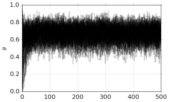
model.run_mcmc(500)
model.plot_chains()
Reading the Output
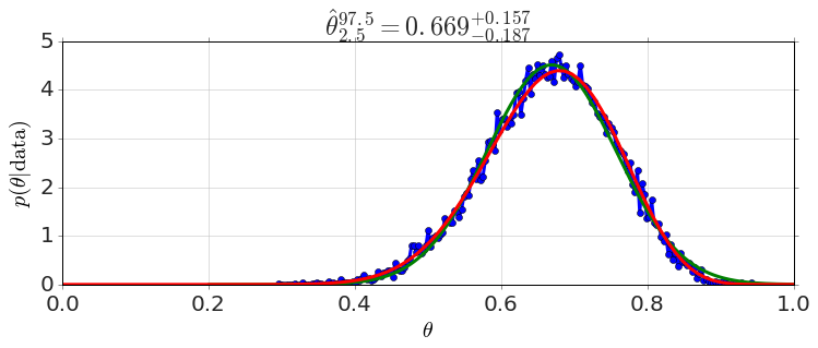
We can now plot the distributions of the parameters, just in this case, yielding best-fits, uncertainties, etc...
model.plot_distributions()(see Figure 11.2)
We can further perform some simple calculations on the probabilities for the parameters, such as
model.P('theta>0.5')Show expected output
0.96173333333333333model.P('(0.2<theta) & (theta<.5)')Show expected output
0.038266666666666664Adapted from Statistical Inference for Everyone, by Brian Blais (Bryant University), licensed under CC BY-SA 4.0 (dual-licensed under the GNU FDL 1.2 or later; this adaptation uses the CC BY-SA grant). Changes were made; this adaptation is distributed under the same license. License: CC-BY-SA-4.0.