7.4 Normal Approximation

The Normal distribution is useful for many reasons: its simple shape, the fact that there are only two parameters which describe it, and the ease with which one can compare the general Normal distribution to the single standard Normal. Further, it can be used as an approximation for several other distributions, under certain limits.

The Beta Distribution

We first saw the beta distribution as the posterior description in a bent-coin parameter estimation problem (see Section 6.4 on page 125 in Chapter 6 (Introduction to Parameter Estimation)). The Normal approximation occurs when the number of flips gets large, compared to how likely the coin flips heads. For notation, we will write the frequency of heads as

$\begin{matrix} f \equiv \frac{h}{N} \end{matrix}$

Normal Approximation to the Beta Distribution The Normal Approximation to the Beta Distribution, for large number of flips ( $N$ ) of which a fraction $f ≡ h / N$ are successful is given by

$\begin{matrix} B e t a (h, N) \sim N o r m a l (μ = f, σ = \sqrt{f (1 - f) / N}) \end{matrix}$

Note

Normal Approximation to the Beta Distribution

The Normal Approximation to the Beta Distribution, for large number of flips ( $N$ ) of which a fraction $f ≡ h / N$ are successful is given by

$\begin{matrix} B e t a (h, N) \sim N o r m a l (μ = f, \\ σ = \sqrt{f (1 - f) / N}) \end{matrix}$

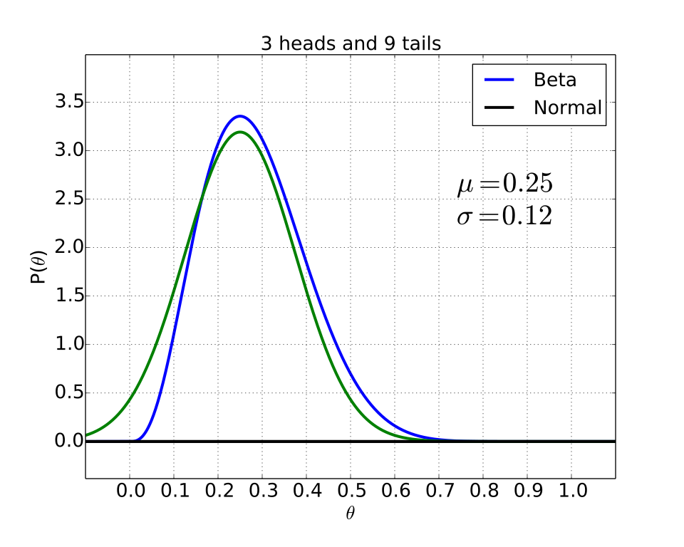
To see how close this approximation can be, observe the following two cases:

Function graph showing y = (x^(0.25*N)*(1-x)^(0.75*N))/(0.25^(0.25*N)*0.75^(0.75*N)) on x in [0, 1] with the region between the curve and the x-axis shaded and y = exp(-(x-0.25)^2*N/0.375). Adjustable parameter: Flips, always one quarter heads (N) = 12. Viewing window: x from -0.22 to 0.76, y from -0.14 to 1.04. — The exact Beta posterior (solid, shaded) against the Normal approximation the box above prescribes (dashed), both scaled to peak height 1, with the fraction of heads held at f = 0.25 throughout. The two cases printed beside this text are two positions of the one slider: N = 12 is the first figure, N = 120 the second. At N = 12 the Beta is visibly lopsided while the Normal is symmetric, and - the point of the margin note - the dashed curve carries real height to the LEFT of theta = 0, assigning probability to a coin that flips heads a negative fraction of the time. The solid curve simply stops there. Drag N up: by 120 the curves are hard to tell apart across the body of the distribution, and by 480 the visible disagreement is gone. Drag it back down and the approximation fails from the tails inward, which is the general rule - a Normal approximation is worst exactly where you were hoping to use it, out at the edges.

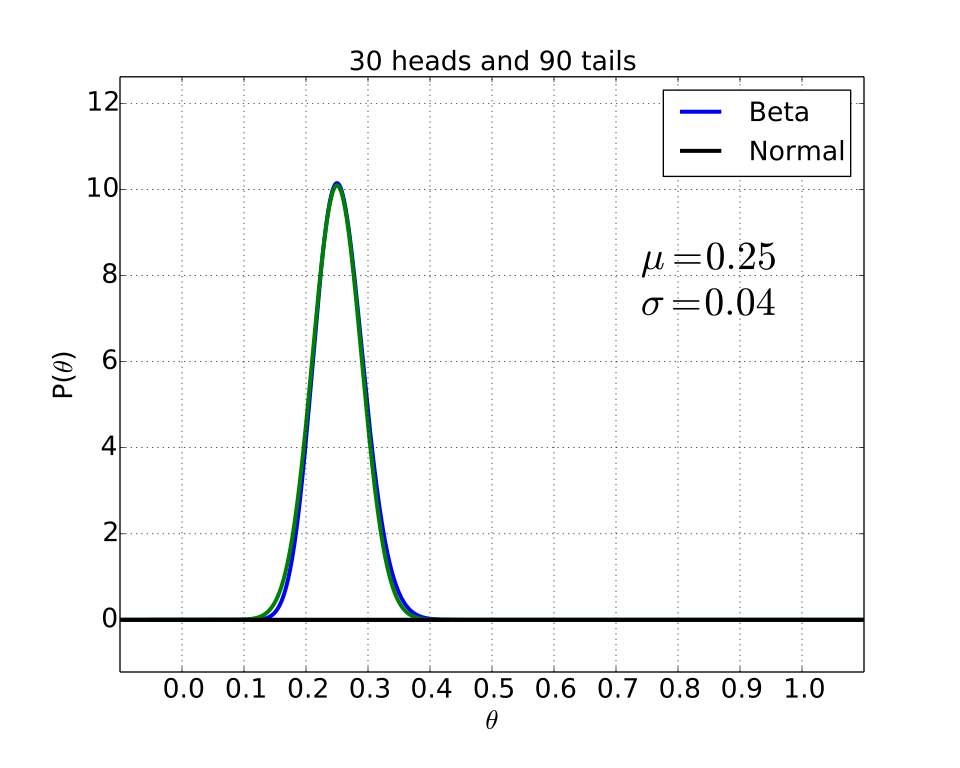
Posterior Beta curve for θ after 3 heads and 9 tails (titled '3 heads and 9 tails') compared with a Normal curve with μ=0.25 and σ=0.12. The two humps roughly agree but the Beta is visibly asymmetric, cut off at θ=0.

With ten times as many flips, we have

Posterior Beta curve for θ after 30 heads and 90 tails compared with a Normal curve with μ=0.25 and σ=0.04; with ten times the data the two curves lie almost exactly on top of each other.

and the curves are so close as to be nearly identical! There still is a (small) probability for getting a negative $θ$ , which is problematic in theory but not typically in practice. To use the properties of the Normal distribution here to quantify our uncertainty about the bent coin. Given 30 heads and 90 tails, the best estimate for $θ$ (i.e. the top of the curve) is 0.25. Our uncertainty is quantified by the width of the distribution, given by $σ$ . Thus, we can be confident to a 95% degree for $θ$ within $2 σ$ , or between 0.17 and 0.33 ( $0.25 - 2 \cdot 0.04$ and $0.25 + 2 \cdot 0.04$ , respectively).

The Binomial Distribution

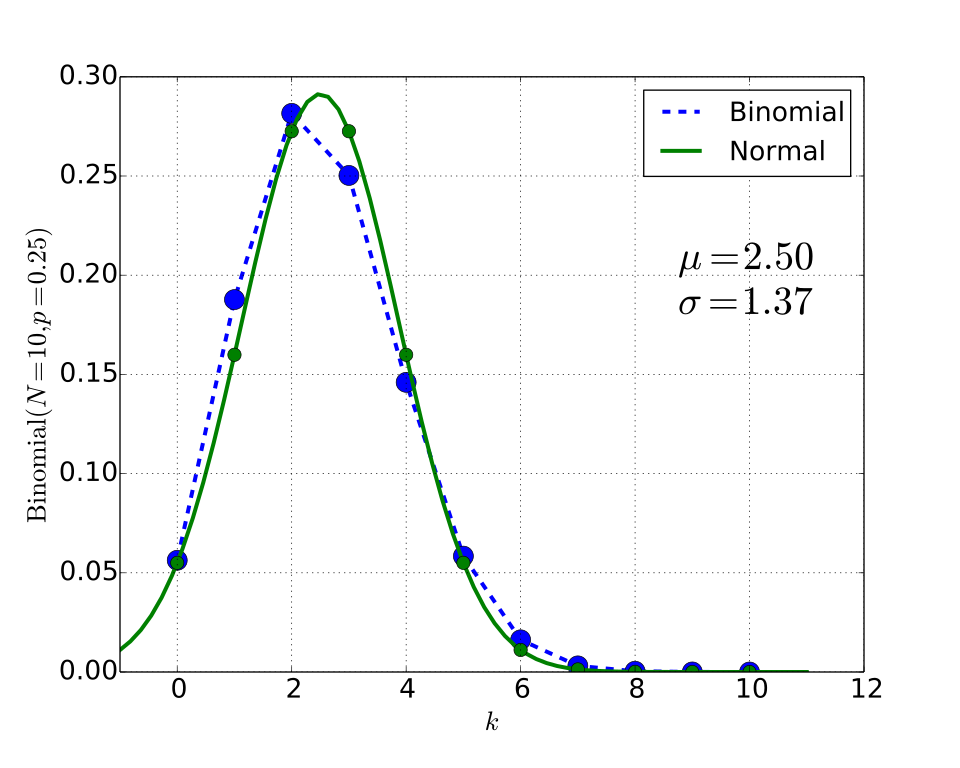
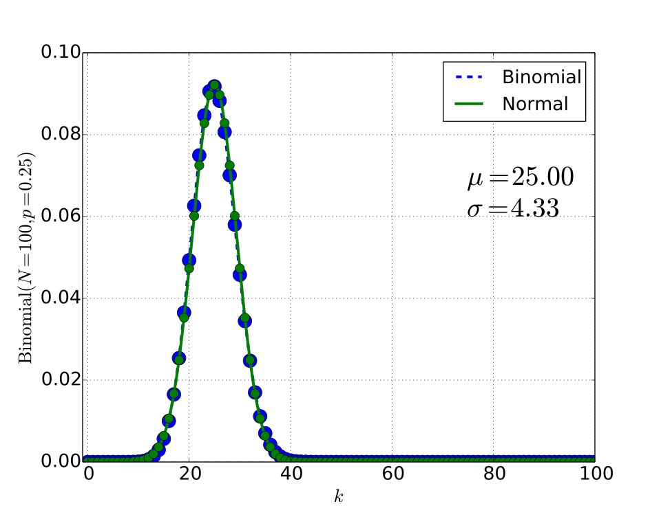
Similarly, with the (discrete) binomial distribution (see Equation 3.3) we have the Normal approximation.

$\begin{matrix} B i n o m i a l (N, p) = N o r m a l (μ = N \cdot p, σ = \sqrt{N \cdot p (1 - p)}) \end{matrix}$

Normal Approximation to the Discrete Binomial Distribution

Note

Normal Approximation to the Discrete Binomial Distribution

$\begin{matrix} B i n o m i a l (N, p) = N o r m a l (μ = N \cdot p, \\ σ = \sqrt{N \cdot p (1 - p)}) \end{matrix}$

with examples

Dots of the Binomial(N=10, p=0.25) distribution versus k overlaid with a solid Normal curve with μ=2.50 and σ=1.37. The Normal approximation tracks the dots closely though both are visibly skewed for this small N.

and

Dots of the Binomial(N=100, p=0.25) distribution versus k overlaid with a Normal curve with μ=25.00 and σ=4.33; at this larger N the dots and the Normal curve are essentially indistinguishable.

The Student's $t$ Distribution

For smallish data sets, $5 less than N less than 30$ , we can replace the estimate of the mean from the Student's $t$ distribution to a Normal distribution with an increased estimate for the deviation. It then becomes practical to use the more convenient $z$ -score to estimate credible intervals rather than the full $t$ tables. The approximation in this domain looks like¹

Normal Approximation to the Student's t Distribution For smallish data sets, $5 less than N less than 30$ ,

$\begin{matrix} {S t u d e n t}_{d o f = N - 1} (\bar{x}, S / \sqrt{N}) \sim N o r m a l (\bar{x}, S k / \sqrt{N}) \\ k \equiv 1 + \frac{20}{N^{2}} \end{matrix}$

Note

Normal Approximation to the Student's t Distribution

For smallish data sets, $5 less than N less than 30$ ,

$\begin{matrix} {S t u d e n t}_{d o f = N - 1} (\bar{x}, S / \sqrt{N}) \sim \\ N o r m a l (\bar{x}, k \cdot S / \sqrt{N}) \\ k \equiv 1 + \frac{20}{N^{2}} \end{matrix}$

Example 1 Estimating the True Length of an Object...Yet Again

Say we have an object, and 5 measurements of its length from the same ruler but from different people,

5.1[ cm], 4.9[ cm], 4.7[ cm], 4.9[ cm], 5.0[ cm]

Unlike earlier, let's say that we don't know the uncertainty (given this ruler) of one measurement. What is the best estimate of the length? Again, the best estimate should be given by the sample mean of these 5 samples,

$\begin{matrix} \hat{μ} = \frac{x_{1} + x_{2} + \dots + x_{N}}{N} \\ = \frac{5.1 [c m] + 4.9 [c m] + 4.7 [c m] + 4.9 [c m] + 5.0 [c m]}{5} = 4.92 [c m] \end{matrix}$

with uncertainty related to the adjusted sample deviation,

$\begin{matrix} S^{2} = \frac{1}{N - 1} ((x_{1} - \bar{x})^{2} + \dots + (x_{N} - \bar{x})^{2}) \\ = \frac{1}{5 - 1} ((5.1 [c m] - 4.92 [c m])^{2} + (4.9 [c m] - 4.92 [c m])^{2} + (4.7 [c m] - 4.92 [c m])^{2} + \\ (4.9 [c m] - 4.92 [c m])^{2} + (5.0 [c m] - 4.92 [c m])^{2}) \\ = 0.024 [c m]^{2} \\ S = \sqrt{0.024 [c m]^{2}} = 0.155 [c m] \\ \frac{S}{\sqrt{N}} = \frac{0.155 [c m]}{\sqrt{5}} = 0.069 [c m] \\ k = 1 + \frac{20}{5^{2}} = 1.8 \\ k \cdot \frac{S}{\sqrt{N}} = 1.8 \cdot 0.069 [c m] = 0.124 [c m] \end{matrix}$

yielding a final best estimate of

$μ hat equals 4.92 open bracket c m close bracket ± 0.124 open bracket c m close bracket$

or (with $2 σ$ range),

$4.92 open bracket c m close bracket, 95 % CI equals open bracket 4.672 open bracket c m close bracket, 5.168 open bracket c m close bracket close bracket$

Compare this range to the one shown in Example 7.5 on page 148. The one here has a slightly larger range, which is a bit more conservative than is needed, but the calculation is quite a bit easier.

Adapted from Statistical Inference for Everyone, by Brian Blais (Bryant University), licensed under CC BY-SA 4.0 (dual-licensed under the GNU FDL 1.2 or later; this adaptation uses the CC BY-SA grant). Changes were made; this adaptation is distributed under the same license. License: CC-BY-SA-4.0.

7.4 Normal Approximation

The Beta Distribution

The Binomial Distribution

The Student's t Distribution

The Student's $t$ Distribution