7.2 The Normal Distribution - Properties

The Normal distribution, also referred to as the Gaussian distribution, is by far the most commonly occurring distribution in all of statistical inference, so it requires some special attention.

The Shape

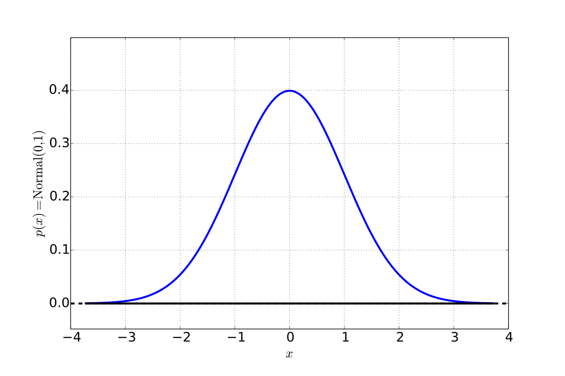
The shape of the Normal distribution is sometimes described as bell-shaped, as shown in Figure 7.1, and is thus referred to as the bell-curve (although there are several other mathematical functions which are bell-shaped). The function is referred to as $N o r m a l (μ, σ)$ where $μ$ and $σ$ are parameters of the model. (see Appendix 14.1 on page 225 for a review of greek letters)

The Normal distribution: a symmetric bell curve labeled p(x)=Normal(0,1), centered at x=0 with peak height about 0.4, falling essentially to zero beyond three units either side. — **Figure 7.1.** The Normal Distribution.

The location parameter, $μ$

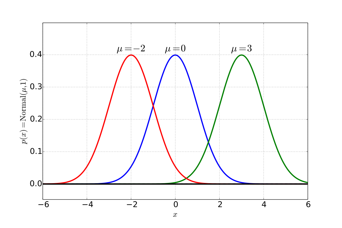
The location parameter (see Figure 7.2) is the value of $x$ for which the Normal distribution has a maximum probability. In a real sense, it is the middle of the distribution, and the best estimate of $x$ . For the Normal distribution the location parameter, $μ$ , is at once the mean, median and mode of the distribution.

The deviation parameter, $σ$

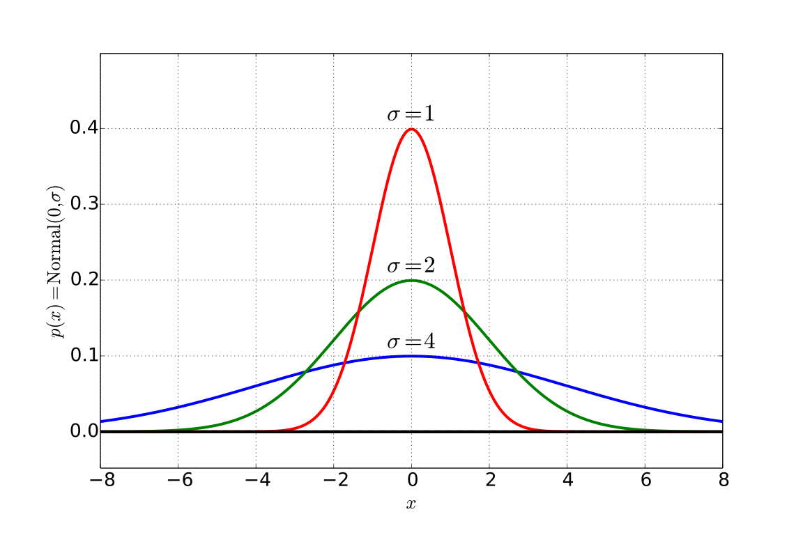
As shown in Figure 7.3 the deviation parameter, $σ$ , is a measure of how spread out the distribution is. As the width increases, the height goes down to keep the area under the curve constant (at 1). As a result, more of the probability sits at larger values of $x$ as $σ$ gets larger.

Three useful properties of $σ$ for the Normal distribution are the following:

the Normal distribution value at the maximum (i.e. at $x = μ$ ) is around 2.7 times larger than the value one- $σ$ away from the maximum (at $x = μ - σ$ and $x = μ + σ$ )
the total probability between these two points is 65%. This is typically written, $μ \pm σ$ .
95% of the distribution lies between $μ minus 2 σ$ and $μ plus 2 σ$ (see Figure 7.3)

For example, writing $5 ± 2$ typically implies a Normal distribution with mean $μ equals 5$ and deviation $σ equals 2$ . One is 65% certain that the range of the estimated value is between 3 and 7, and 95% certain that the range is between 1 and 9 (i.e. mean minus two deviations and mean plus two deviations).

Three Normal curves centered at zero with different widths: σ=1 is tall and narrow (peak 0.4), σ=2 is half as tall and twice as wide, and σ=4 is a low broad mound (peak 0.1). Larger deviation spreads the same total probability over a wider range. — **Figure 7.3.** The Normal distribution with different deviation parameters, $σ$ .

Summarizing the Distribution

We can specify the Normal distribution with just the two parameters, $μ$ and $σ$ - the location and deviation parameters, respectively. However, due to its symmetry, we can summarize this distribution for all cases by looking a a single special case called the standard Normal distribution.

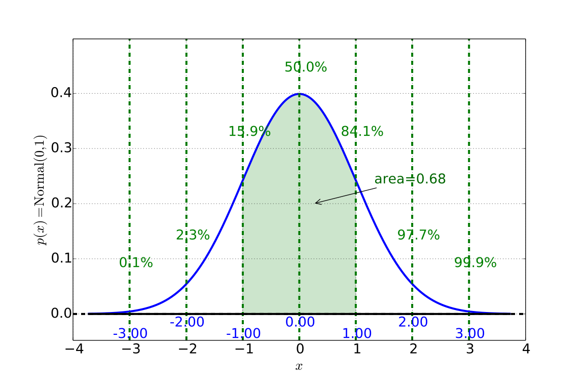
The Standard Normal Distribution is the Normal distribution in the special case where $μ equals 0$ (the distribution is centered at $x equals 0$ ) and $σ equals 1$ (the distribution has a spread of 1).

For any Normal distribution, the area within 1- $σ$ is 0.68, within 2- $σ$ is 0.95, and 3- $σ$ is 0.99. These locations are the most prevalently used in any kind of statistical testing, and thus we will see them many times.

The standard Normal curve with dashed vertical lines at -3, -2, -1, 0, 1, 2 and 3, each labeled with the percentile of the area to its left: 0.1%, 2.3%, 15.9%, 50%, 84.1%, 97.7% and 99.9%. The shaded band between -1 and +1 is annotated 'area=0.68'. — **Figure 7.4.** The Standard Normal Distribution (the Normal distribution in the special case where $μ equals 0$ and $σ equals 1$ ). The percentiles shown are for positions 1- $σ$ away from the center, 2- $σ$ away, and 3- $σ$ away. The area within 1- $σ$ is 0.68, within 2- $σ$ is 0.95, and 3- $σ$ is 0.99. These locations are the most prevalently used in any kind of statistical testing, and thus we will see them many times.

Moving from a General Normal to the Standard Normal and Back

In order to use the table of percentiles for the standard Normal distribution, we need to be able to translate from the Normal to the standard Normal and back again. Luckily, it is a simple process, and is one of the main reasons for using the Normal distribution - other distributions are not so easily manipulated.

To facilitate this translation, we will use the variable $x$ for the Normal distribution and $z$ for the standard Normal. So now, we need to have a recipe for translating $x$ to $z$ (or vice versa), given $μ$ and $σ$ . These recipes are:

$x$ to $z$ : subtract $x$ by $μ$ , and divide by $σ$
$z$ to $x$ : multiply $z$ by $σ$ and add $μ$

Example 2 Given a Normal distribution with a mean of $μ equals 150$ and $σ equals 30$ , what is the probability $P open parenthesis x greater than 170 close parenthesis$

To use the tables in Section 16.3 on page 238, we first need to translate everything to the standard Normal values.

$\begin{matrix} x = 170 \Rightarrow z = \frac{x - 150}{30} = 0.67 \end{matrix}$

From the table in Section 16.3 on page 238, the area to the left of $z equals 0.67$ is 0.7486. Because we are asked the probability greater than $x equals 170$ we need to have the area to the right of the curve, or

$\begin{matrix} P (x > 170) = 1 - 0.7486 = 0.2514 \end{matrix}$

or about 1/4. In other words, with a mean $μ equals 150$ and deviation $σ equals 20$ , we'd expect about a quarter of the time that the value of the variable would be greater than 170. Or, given our uncertainty of a specific value, we'd assign a probability of around 25% to it being larger than 170.

Sum and Differences

One more convenient property of the Normal distribution is that sums and differences of variables that individually have Normal distributions also have Normal distributions, although each with a different mean and deviation parameter. The relationships are summarized as follows.

Sum of two Normally distributed variables If we have two variables, $x$ and $y$ , which have Normal distributions

$\begin{matrix} P (x) = N o r m a l (μ_{x}, σ_{x}) \\ P (y) = N o r m a l (μ_{y}, σ_{y}) \end{matrix}$

then their sum, $x + y$ , has a mean the sum of the two, $μ_{x} + μ_{y}$ and a deviation $\sqrt{σ_{x}^{2} + σ_{y}^{2}}$ .

Note

Sum of two Normally distributed variables

If we have two Normally distributed variables, $x$ and $y$ , we have

$\begin{matrix} P (x) = N o r m a l (μ_{x}, σ_{x}) \\ P (y) = N o r m a l (μ_{y}, σ_{y}) \\ P (x + y) = N o r m a l (μ_{x} + μ_{y}, \\ \sqrt{σ_{x}^{2} + σ_{y}^{2}}) \end{matrix}$

One way to remember this is that the new squared deviation parameter is the sum of the two old ones,

$\begin{matrix} σ_{x + y}^{2} = σ_{x}^{2} + σ_{y}^{2} \end{matrix}$

Differences between two Normally distributed variables For differences, $x - y$ , we have a new mean of $μ_{x} - μ_{y}$ and deviation parameter again $\sqrt{σ_{x}^{2} + σ_{y}^{2}}$ . Note the “+” sign in the new $σ$ , which keeps the new $σ$ positive which is must be by definition.

Note

Differences between two Normally distributed variables

$\begin{matrix} P (x - y) = N o r m a l (μ_{x} - μ_{y}, \\ \sqrt{σ_{x}^{2} + σ_{y}^{2}}) \end{matrix}$

(Note the “+” sign in the new $σ$ .)

If we are asked for the distribution of a quantity with an added constant, like

$\begin{matrix} z = x + c o n s t a n t \end{matrix}$

then the probability of $z$ is just the same as that of $x$ (i.e. Normal distribution with the same deviation), with the location parameter moved by the constant

$\begin{matrix} P (z) = N o r m a l (μ_{x} + c o n s t a n t, σ_{x}) \end{matrix}$

Adapted from Statistical Inference for Everyone, by Brian Blais (Bryant University), licensed under CC BY-SA 4.0 (dual-licensed under the GNU FDL 1.2 or later; this adaptation uses the CC BY-SA grant). Changes were made; this adaptation is distributed under the same license. License: CC-BY-SA-4.0.