7D Systems of Linear Equations

Read the transcript Download the video Narration credits and licences

Companies often look at more than one equation of a line when analyzing how their business is doing. For example a company might look at a cost equation and a revenue equation. The number of items the company needs to make so that the costs and revenue are the same is often called the break-even point. But how can we figure out the break-even point when we have two different equations? This is one of the many applications of Linear Systems.

Three Types of Linear Systems

When two lines are drawn on a graph three things can happen. Either the lines will meet at a point, the lines will be distinct parallel lines and not meet, or the two lines happen to be the same line and would have all their points in common. These three things correspond to the three types of linear systems. The key is that the solutions are only points that lie on both lines.

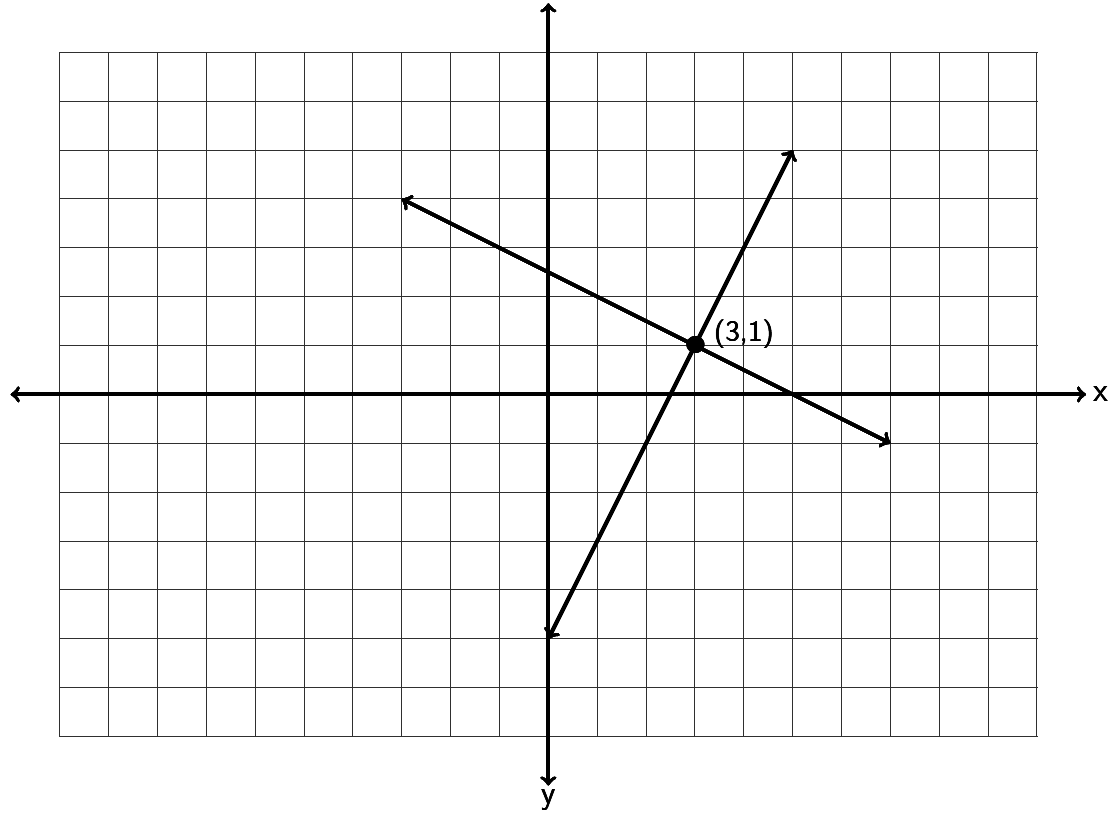
In a system where the two lines intersect at a point, the one ordered pair (x,y) where the lines meet is the solution we are looking for. Many books call this an independent system of equations or an independent system for short. In the example below, the solution is (3,1).

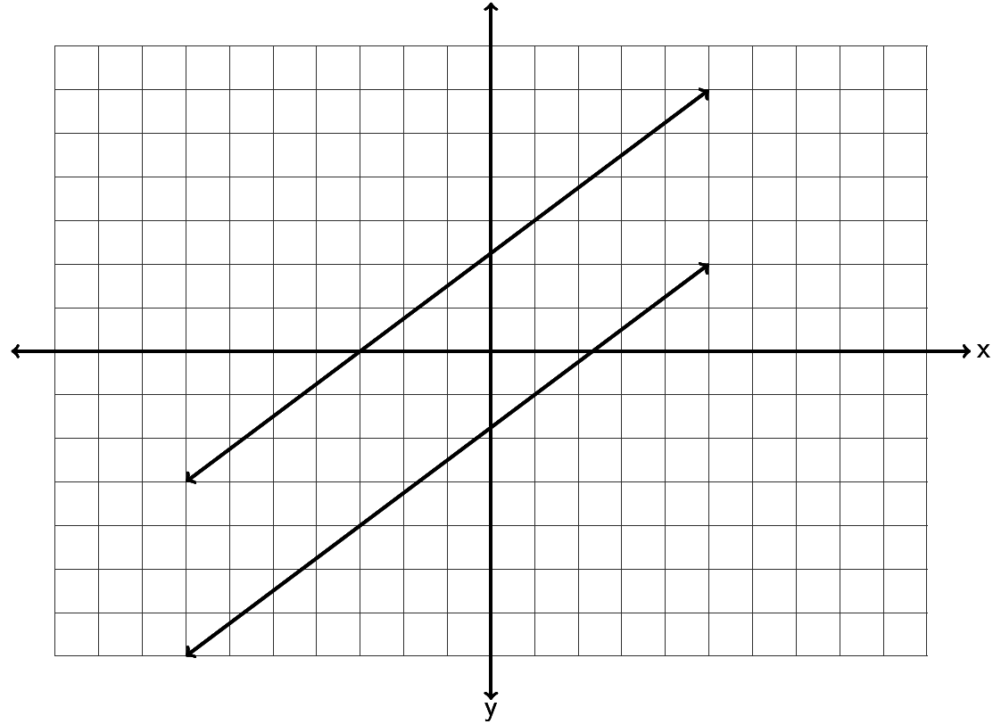
Coordinate axes with one ascending and one descending line intersecting at the labelled point (3, 1).

In a system where the two lines are distinct parallel lines, we see that the lines never meet and no points lie on both lines. So there is “no solution” when the lines are parallel. Many books call this an inconsistent system.

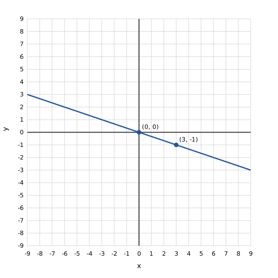
Coordinate axes with two distinct parallel ascending lines. They cross the y-axis at different heights and never meet.

In a system where the two lines happen to be the same line, the two lines have all their points in common. When this happens, the solution is “All points on the line are solutions.” Many books call this a dependent set of equations or a dependent system for short. Notice a dependent system has infinitely many solutions.

Illustrative coordinate grid with one shared descending line representing two coincident lines. Every point on the shared line is a solution. The plotted example uses y=-x/3; marked points (0,0) and (3,-1) illustrate the shared line.

Solving a System by Graphing

To find the solution to a system, we can graph both lines and see if and where they meet. For example, solve the following system by graphing.

$\begin{array}{l} y = 3 x - 7 \\ y = \frac{1}{2} x - 2 \end{array}$

Since both equations are in slope-intercept form, we can use the slope and y-intercept to graph each line. The first line has a slope of 3/1 and a y-intercept of (0,-7). So we can start at -7 on the y-axis and go up 3 and right 1. The second line has a slope of ½ and a y-intercept of (0,-2). So we can start at -2 on the y-axis and go up 1 and right 2.

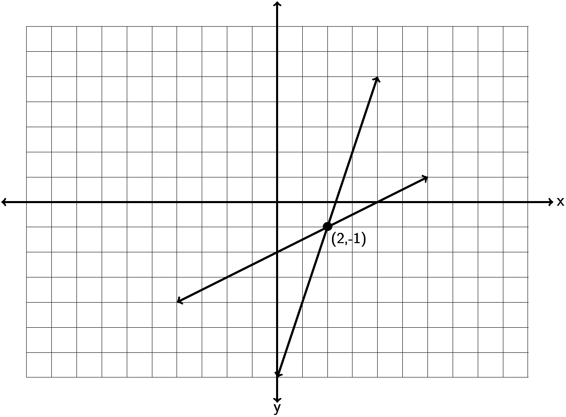
Coordinate axes with two ascending lines of different steepness intersecting at the labelled point (2, -1).

So do the lines intersect and if so where do they intersect? Notice the lines intersect at (2, -1) so that is the solution to the system. To check the answer plug in 2 for x and -1 for y into both equations. If it makes both equations true, it is the solution.

$\begin{array}{l} y = 3 x - 7 y = \frac{1}{2} x - 2 \\ - 1 = 3 (2) - 7 - 1 = \frac{1}{2} (2) - 2 \\ - 1 = 6 - 7 - 1 = 1 - 2 \\ - 1 = + 6 + - 7 - 1 = + 1 + - 2 \\ - 1 = - 1 True! - 1 = - 1 True! \end{array}$

Let’s try another example. Solve the following system by graphing.

$\begin{array}{l} 5 x + 2 y = 10 \\ y = - \frac{5}{2} x + 5 \end{array}$

Since the first line is not in slope-intercept form, we can graph it by finding the x and y-intercepts. Plugging in 0 for x gives 2y=10 which gives y = 5. So the y-intercept is (0,5). Plugging in y = 0 we get 5x = 10 which gives x = 2. So the x-intercept is (2,0). We can plot (0,5) and (2,0) and draw the line.

The second line is in slope-intercept form, so we can see the y-intercept is (0,5) and the slope is -5/2. So we will start at 5 on the y-axis and go down 5 and right 2. If you notice this coincides perfectly with the first line we drew.

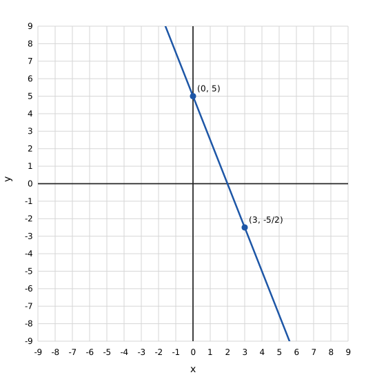
Coordinate grid showing the shared descending line y=-5x/2+5. It represents both 5x+2y=10 and y=-5x/2+5. Marked points (0,5) and (3,-5/2) lie on the shared line; its x-intercept is (2,0).

So the two equations we graphed were actually the same line. Since the lines have all their points in common, the solution is “All points on the line are solutions.”

$\begin{array}{rcl} 5 x + 2 y & = & 10 \\ - 5 x & - 5 x \\ 0 + 2 y & = & - 5 x + 10 \\ 2 y & = & - 5 x + 10 \\ \frac{{}^{1}2 y}{2} & = & \frac{- 5 x + 10}{2} \\ y & = & \frac{- 5 x}{2} + \frac{{}^{5}10}{2} \\ y & = & - \frac{5}{2} x + 5 \end{array}$

Since both equations have the exact same slope and the exact same y-intercept, they are in fact the exact same line and will have all their points in common.

Look at this example. Solve the following system of equations by inspection. (Just look at the slopes and y-intercepts.)

$\begin{array}{l} y = \frac{1}{3} x - 4 \\ y = \frac{1}{3} x + 6 \end{array}$

Notice both equations are in slope-intercept form. Notice they both have the same slope but different y-intercepts. If you recall from the section on slope, these lines are parallel. Notice they have the same slope but they definitely are not the same line. Since the lines are parallel, they will never intersect and the solution to the system is “No Solution.”

Solve the following systems with your instructor either by graphing or by inspection.

Solving linear systems by substitution

If you do not want to solve the system by graphing, there is a way to figure out the answer with algebra. The method is called the “substitution method”. Here are the steps to the substitution method.

Steps to solving a system with Substitution

Solve one of the equations for one of the variables. (It can be x or y in either equation. If one of your equations is already in slope-intercept form, then you can just use the y in that equation.)
Plug in (substitute) the value of the variable in step 1 into the other equation you have not used yet. (You should be left with an equation with only one letter in it.)
Solve the one-variable equation. (If the system only has one ordered pair as the answer, then this will give you either the x or y-coordinate of the answer.)
Plug in the value of the variable solved for in step 3 into any of the equations and solve for the remaining variable that you don’t know.
Check your ordered pair answer by plugging into both equations and seeing if they both make true statements.

Look at the following example. Solve the following system with the substitution method.

$\begin{array}{l} 2 x + 3 y = 3 \\ x - 5 y = 8 \end{array}$

Step 1: Solve for one of the letters. Since you can choose any variable, choose something easy to solve for. (x in equation 2 looks easy)

$\begin{array}{rcl} x - 5 y & = & 8 \\ + 5 y & + 5 y \\ x & = & 5 y + 8 \end{array}$

Step 2: Now plug in 5y+8 for x in the other equation. Notice the equation only has one letter now.

$\begin{array}{l} 2 x + 3 y = 3 \\ 2 (5 y + 8) + 3 y = 3 \end{array}$

Step 3: Solve the one-variable equation. Notice we need to use the distributive property.

$\begin{array}{rcl} 2 (5 y + 8) + 3 y & = & 3 \\ 10 y + 16 + 3 y & = & 3 \\ 13 y + 16 & = & 3 \\ - 16 & - 16 \\ 13 y + 0 & = & - 13 \\ \frac{{}^{1}13 y}{13} & = & \frac{{}^{- 1}{- 13}}{13} \\ y & = & - 1 \end{array}$

Step 4: We know that our answer is $open parenthesis ? ? ?, minus 1 close parenthesis$ . We will plug in -1 for y into any of the equations with two variables and solve. Any equation you use will give you the same answer for x.

$\begin{array}{rcl} x - 5 y & = & 8 \\ x - 5 (- 1) & = & 8 \\ x + 5 & = & 8 \\ - 5 & - 5 \\ x & = & 3 \end{array}$

Step 5: So our answer is $open parenthesis 3, minus 1 close parenthesis$ . Let’s check the answer by plugging in 3 for x and -1 for y into both equations and see if both of them are true.

$\begin{array}{l} 2 x + 3 y = 3 x - 5 y = 8 \\ 2 (3) + 3 (- 1) = 3 3 - 5 (- 1) = 8 \\ 6 - 3 = 3 True!! 3 + 5 = 8 True!! \end{array}$

Try the following examples of solving with the substitution method with your instructor.

Practice Problems Section 7D

Solve the following linear systems by inspection. (Hint: Examine the slope and y-intercepts.) You do not have to do any work for these. Just give the solution to the system.

$\begin{array}{l} y = - \frac{3}{4} x + 19 \\ y = - \frac{3}{4} x - 12 \end{array}$
$\begin{array}{l} y = 4 x - 5 \\ y = 4 x - 5 \end{array}$
$\begin{array}{l} y = 5 x + 7 \\ y = - \frac{1}{3} x + 7 \end{array}$
$\begin{array}{l} y = \frac{2}{5} x + 1 \\ y = \frac{2}{5} x - 8 \end{array}$
$\begin{array}{l} y = - 2 x - 6 \\ y = - \frac{1}{4} x - 6 \end{array}$
$\begin{array}{l} y = - \frac{4}{7} x - 2 \\ y = - \frac{4}{7} x - 2 \end{array}$

Solve the following linear systems by graphing both lines. You must graph both lines and give the solution to the system.

$\begin{array}{l} y = - 3 x + 9 \\ y = - \frac{1}{4} x - 2 \end{array}$
$\begin{array}{l} y = \frac{2}{3} x + 3 \\ y = - \frac{1}{2} x - 4 \end{array}$
$\begin{array}{l} x + 3 y = - 3 \\ y = - \frac{1}{3} x + 4 \end{array}$
$\begin{array}{l} y = 1 x + 4 \\ y = - 1 x + 0 \end{array}$
$\begin{array}{l} 4 x - 6 y = 0 \\ y = \frac{2}{3} x + 0 \end{array}$
$\begin{array}{l} y = - 2 x + 3 \\ 6 x + 3 y = - 3 \end{array}$

Solve the following linear systems by using the substitution method.

$\begin{array}{l} 3 x + 4 y = - 1 \\ - 2 x + 5 y = - 7 \end{array}$
$\begin{array}{l} y = - 3 x + 26 \\ y = - \frac{1}{4} x + 4 \end{array}$
$\begin{array}{l} 2 x - y = - 1 \\ 3 x + 4 y = - 29 \end{array}$
$\begin{array}{l} y = \frac{1}{2} x + \frac{9}{2} \\ y = \frac{3}{5} x - 5 \end{array}$
$\begin{array}{l} y = 1.4 x + 1.6 \\ y = - 2.3 x + 5.3 \end{array}$
$\begin{array}{l} 0.3 x + 0.5 y = 6.5 \\ 0.04 x + 0.1 y = 1.2 \end{array}$

Adapted from Preparing for Algebra and Statistics, Third Edition, by Matt Teachout. License: CC BY 4.0. Copyright and sources.