5.3 Conservative Fields

A vector field assigns an arrow $𝐅 (x, y) = (P, Q)$ to every point — a wind map, a force map. The natural integral of a field is work: along a curve $C$ traced by $𝐫 (t)$ ,

$\int_{C} 𝐅 \cdot d 𝐫 = \int_{a}^{b} 𝐅 (𝐫 (t)) \cdot 𝐫^{'} (t) d t,$

which totals the field's push along your direction of travel. The deepest question you can ask about a field is whether it is somebody's gradient: $𝐅 equals ∇ f$ for a potential $f$ . Such conservative fields inherit a fundamental theorem — work equals potential difference, $f (end) - f (start)$ — so work is path-independent, and around any closed loop it is exactly zero. One loop is therefore a courtroom: the figure puts two fields on trial.

A flat carpet of arrows seen from almost straight overhead, crossed by a dark circle of radius 1.5 centered at the origin. The visible field's arrows all point radially outward, brightening from purple to yellow away from the center, so along the dark circle they cross it at right angles everywhere; a second, hidden field can be toggled visible in its place, whose arrows instead circulate counterclockwise and run along the circle rather than across it. Comparing how each field meets the loop is the scene's whole game: crossing everywhere means zero circulation, running along it means circulation that never cancels. 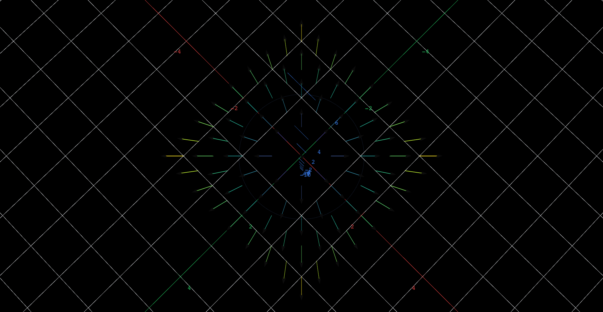— An overhead view of a flat carpet of arrows crossed by a dark circle of radius $1.5$ centered at the origin. The visible field $𝐅 equals open parenthesis 2 x, 2 y close parenthesis$ points radially outward everywhere, its arrows brightening from purple to yellow with distance from the center. A second field, $𝐅 = (- y, x)$ , hides in the object list; toggled visible in its place, its arrows circulate counterclockwise, running *along* the circle instead of across it.

Explore

Follow the dark circle with your eye. The visible field's arrows cross it at a right angle at every single point — the field has no component along the walk anywhere. Predict the circulation around the loop before computing it.
Hide the radial field and reveal the rotational one with their eye toggles. Now the arrows run along the circle: at every point of a counterclockwise walk, the field is at your back. Can contributions like that cancel? Predict this circulation's sign.
Both fields have constant strength on the circle — the arrows along it share one color. Compute the two strengths at radius $1.5$ by hand and check which field's arrows sit further toward yellow.
The radial field is a gradient: find, by inspection, a function $f$ with $∇ f equals open parenthesis 2 x, 2 y close parenthesis$ , and describe its graph. Walking any closed loop on that surface, why must you end at the height you started?
Try the same for $(- y, x)$ : what would $f_{x} = - y$ and $f_{y} = x$ demand of the mixed second derivatives $f_{y x}$ and $f_{x y}$ ? Clairaut's theorem says those must be equal for any twice-differentiable $f$ — conclude what the example below confirms by direct integration.

[2 \cdot x, 2 \cdot y]

∇f for the potential f = x² + y² ✓ Computed · mojocas 0.1.0 ✓ Agrees with the text

Step 4 asks you to find a potential by inspection. This is the check: the gradient of $f = x^{2} + y^{2}$ is exactly the radial field the figure draws, so that field is conservative and the loop integral must vanish.

[\begin{matrix} 0 & - 1 \\ 1 & 0 \end{matrix}]

The derivative matrix of the rotational field ✓ Computed · mojocas 0.1.0

Step 5's argument, computed. If $(- y, x)$ were $∇ f$ , this matrix would be $f$ 's Hessian — and Clairaut's theorem forces a Hessian to be symmetric. The off-diagonal entries are $minus 1$ and $1$ . They differ, so no such $f$ exists and the rotational field cannot be conservative, no potential-hunting required.

The verdict, computed both ways

For a conservative field the fundamental theorem for line integrals does all the work, and the geometric tell is the one in step 1: a gradient field crosses its own potential's level curves squarely (Chapter 4), so against a loop that happens to be a level curve it musters no push at all. The rotational field fails a cheaper test: comparing cross-partials, $\partial Q / \partial x - \partial P / \partial y = 1 - (- 1) = 2 \neq 0$ , while every gradient field must score zero there. But the most honest verdict is a line integral, computed below — and its value is worth keeping: the same number returns in the next section wearing a theorem.

Example 1 Two fields, one loop, two verdicts

Compute the circulation of $𝐅 equals open parenthesis 2 x, 2 y close parenthesis$ and of $𝐅 = (- y, x)$ counterclockwise around the circle $𝐫 open parenthesis t close parenthesis equals open parenthesis 1.5 cos t, 1.5 sin t close parenthesis$ , $t ∈ [ 0, 2 π ]$ .

The velocity is $𝐫^{'} (t) = (- 1.5 \sin t, 1.5 \cos t)$ . For the radial field, $𝐅 open parenthesis 𝐫 open parenthesis t close parenthesis close parenthesis equals open parenthesis 3 cos t, 3 sin t close parenthesis$ , so

$𝐅 \cdot 𝐫^{'} = - 4.5 \sin t \cos t + 4.5 \sin t \cos t = 0$

at every $t$ : the integrand is identically zero and the circulation is $0$ — perpendicularity, in numbers. Consistently, $𝐅 equals ∇ f$ for $f = x^{2} + y^{2}$ (check: $f sub x equals 2 x$ , $f sub y equals 2 y$ ), and a closed loop on the bowl $f$ ends at its starting height. For the rotational field, $𝐅 (𝐫 (t)) = (- 1.5 \sin t, 1.5 \cos t)$ , which is exactly $𝐫^{'} (t)$ : the field rides the walk perfectly, and

$𝐅 \cdot 𝐫^{'} = 2.25 \sin^{2} t + 2.25 \cos^{2} t = 2.25,$

a constant. The circulation is $2.25 \cdot 2 π = 4.5 π \neq 0$ — so $(- y, x)$ is not conservative, no potential exists, and the cross-partials test's nonzero score of $2$ was telling the truth. Note $2.25$ is the squared radius: this field's circulation grows with the loop, a hint the next section explains.

An original work of XYZ Homework, built around interactive XYZ 3D figures. Aligned to OpenStax Calculus Volume 3 (Strang & Herman), © OpenStax (Rice University), licensed CC BY-NC-SA 4.0; no OpenStax content is reproduced, and this work is not affiliated with or endorsed by OpenStax or Rice University. License: CC-BY-NC-SA-4.0.