5.2 Change of Variables

The last section earned one correction factor, the polar $r$ , by measuring mesh cells. This section is the same idea with the training wheels off. A change of variables is a map

$T (u, v) = (x (u, v), y (u, v))$

that carries a simple region in the $u v$ -plane — ideally a square — onto the region you actually care about. Chop the square into a grid and $T$ carries the grid along: the image is a curvilinear mesh, and each little square cell lands as a little curvilinear cell whose area has been scaled by some local factor. That factor is the Jacobian determinant, and the figure puts it under two sliders.

Seen from almost straight overhead, a faint gray wireframe unit square sits in the plane, and over it lies a brightly colored curvilinear quadrilateral: the image of that square under the map T(u, v) = (u + a v, v + b u squared), carrying a mesh of small cells that stretch and shrink from one corner of the region to the other. Slider a shears the top edge sideways and slider b bends the bottom edge into a parabola; setting both sliders to zero makes the colored image coincide with the gray square, and the varying cell sizes elsewhere are the Jacobian made visible. 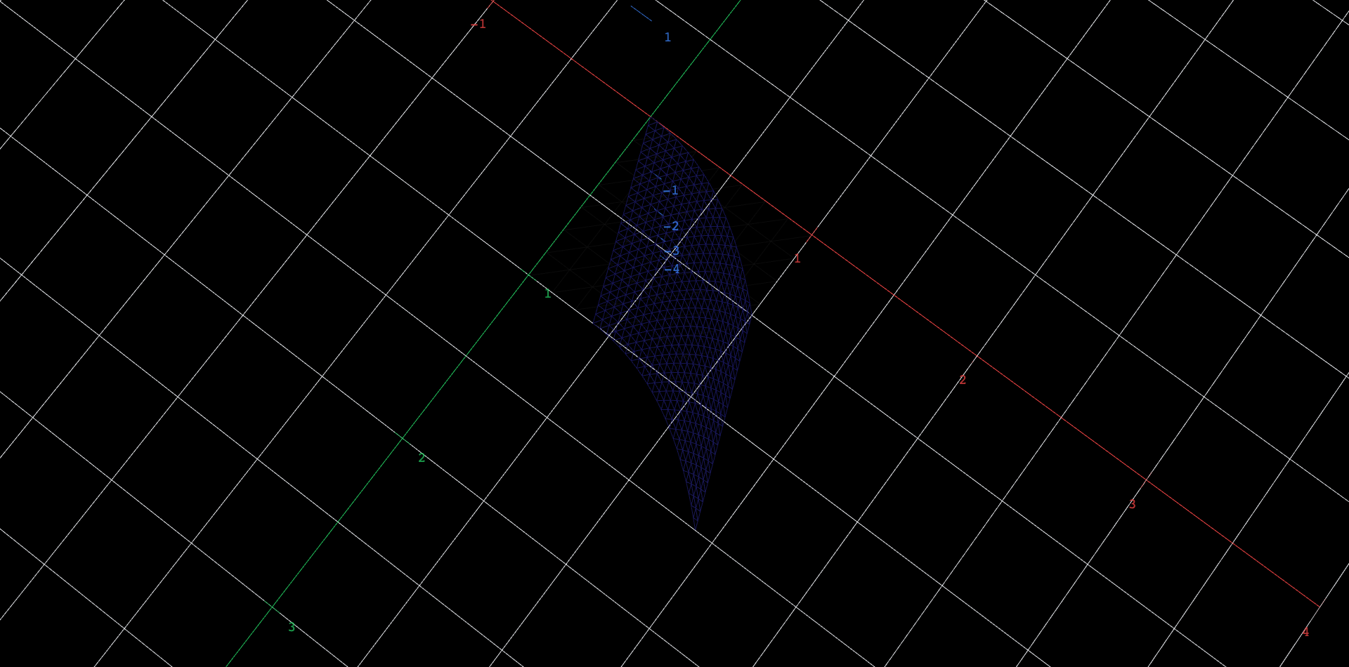— Seen from nearly overhead: a faint gray wireframe unit square, and over it the brightly colored curvilinear image of that square under $T (u, v) = (u + a v, v + b u^{2})$ , carrying a fine mesh of cells. Slider $a$ (shear strength, $minus 1$ to $1$ , starting at $0.4$ ) skews the square sideways; slider $b$ (bend strength, $minus 1$ to $1$ , starting at $0.5$ ) bows its bottom edge into a parabola. With both sliders at zero the colored image coincides with the gray square.

Explore

Set both sliders to $0$ and confirm the image is the unit square, every cell congruent. This is the identity map; its Jacobian should be $1$ everywhere.
Raise $a$ alone. The square shears sideways into a parallelogram — but look closely at the cells. Are they still all the same size? A shear slides rows past each other without compressing them; predict the Jacobian of a pure shear, then check against the formula below.
Return $a$ to $0$ and raise $b$ alone. The bottom edge bows into a parabola and cells tilt — but do they change area? Sliding each column vertically by $b u^{2}$ is a shear too, just a vertical one.
Now set the sliders to their starting values $a equals 0.4$ , $b equals 0.5$ , where both effects act at once. The cells are no longer equal: find where in the mesh they are smallest. Is it along the $u equals 0$ edge or the $u equals 1$ edge of the image?
Push both sliders to $1$ and watch the mesh pinch: cells collapse toward zero area along a band in the middle of the region, and beyond it the mesh folds back over itself. The formula below says the Jacobian there passes through zero and changes sign — a warning that $T$ has stopped being one-to-one, which honest substitutions must not do on the interior.

The Jacobian is the cell-area scale

Near a point $(u, v)$ , the map $T$ acts like its linear approximation: the mesh cell with sides $Δ u$ and $Δ v$ lands as a small parallelogram whose area is $| J open parenthesis u, v close parenthesis | Δ u Δ v$ , where

$J (u, v) = \frac{\partial x}{\partial u} \frac{\partial y}{\partial v} - \frac{\partial x}{\partial v} \frac{\partial y}{\partial u} .$

Summing function values against these true cell areas and refining gives the change-of-variables formula:

$∬ sub R f open parenthesis x, y close parenthesis d A equals ∬ sub S f open parenthesis T open parenthesis u, v close parenthesis close parenthesis | J open parenthesis u, v close parenthesis | d u d v,$

where $T$ carries $S$ one-to-one onto $R$ . The polar map $T (r, θ) = (r \cos θ, r \sin θ)$ is the marquee special case: its Jacobian is $\cos θ \cdot r \cos θ - (- r \sin θ) \cdot \sin θ = r$ , and the last section's area element falls out of the general machine.

Example 1 The Jacobian of the two-slider map, and the image's area

For $T (u, v) = (u + a v, v + b u^{2})$ , compute the Jacobian determinant, explain what you saw at the sliders' settings in the Explore steps, and find the exact area of the image of the unit square when $a equals 0.4$ , $b equals 0.5$ .

The four partials are $∂ x / ∂ u equals 1$ , $∂ x / ∂ v equals a$ , $∂ y / ∂ u equals 2 b u$ , $∂ y / ∂ v equals 1$ , so

$J (u, v) = (1) (1) - (a) (2 b u) = 1 - 2 a b u .$

With $b equals 0$ (pure horizontal shear) or $a equals 0$ (pure vertical shear), $J equals 1$ everywhere — shears preserve area, as steps 2 and 3 showed. With $a equals 0.4$ , $b equals 0.5$ we get $J = 1 - 0.4 u$ : positive on the whole square but smallest at $u equals 1$ , which is why the cells shrink toward that edge of the image (step 4). And with $a = b = 1$ , $J = 1 - 2 u$ hits zero at $u = \frac{1}{2}$ — the pinch line of step 5 — and is negative beyond, the algebraic trace of the fold. The image's area is the integral of the scale factor:

$\int_{0}^{1} \int_{0}^{1} (1 - 0.4 u) d u d v = 1 - 0.4 \cdot \frac{1}{2} = 0.8 .$

The colored region really is 20 percent smaller than the gray square it came from — the mesh told you where the shrinkage lives, and the Jacobian told you exactly how much.

An original work of XYZ Homework, built around interactive XYZ 3D figures. Aligned to OpenStax Calculus Volume 3 (Strang & Herman), © OpenStax (Rice University), licensed CC BY-NC-SA 4.0; no OpenStax content is reproduced, and this work is not affiliated with or endorsed by OpenStax or Rice University. License: CC-BY-NC-SA-4.0.